Systematic management and analysis of yeast gene expression data

John Aach, Wayne Rindone, and George M. Church

Department of Genetics, Harvard Medical School, 200 Longwood Ave., Boston, MA, 02115, USA

and

Lipper Center for Computational Functional Genomics, 77 Louis Pasteur Avenue, Boston, MA 02115, USA

January 26, 2000

In this supplement we report results of work pertaining to the generation and comparison through condition clustering of Estimated Relative Abundances (ERAs) developed for 154 yeast microarray conditions on ExpressDB. These results were not described in the article. The data sets involved are listed in Table 1 of the main text of the article. We also describe an alternative clustering of ERA data than the one discussed in the article (Figure 4). Note that references to experimental data sets in this supplement use series codes listed in Table I (e.g., Der_diaux = diauxic shift data reported in (DeRisi et al., 1997)). Note also that this supplement contains a Methods section that is supplemental to that given in the article. To distinguish references to the article Methods section from this supplement's Methods section, the latter will be referred to here as "Supplemental Methods" and the former simply as "Methods."

• Generation of microarray-derived Estimated Relative Abundances
• Clustering of microarray experimental conditions
• Discussion
• Supplemental Methods
• Figures
• Figure 3: Results of clustering 217 conditions by Pearson correlation coefficients over 1078 ORFs
• Figure 4: Results of clustering 958 high expressing ORFs over 213 conditions, with clustering both by ORF and by condition
• Figure 5: Portion of dendrogram of clustering of Figure 4 that contains diauxic shift and sporulation condition series
• Figure 6: Comparison of condition clusterings of diauxic shift and sporulation time course experiment series based on microarray ratios vs. ERAs
• References
• Copyright

Generation of microarray-derived Estimated Relative Abundances

As noted in the text of the article, generation of ERAs for microarray data is difficult because microarray results are reported as ratios of expression levels in an experimental condition relative to a control condition. Under the assumption that the total number of mRNAs stays roughly constant across conditions these may be considered ratios of ERAs for two conditions, and the individual control and experimental condition ERAs cannot be recovered unless one of them can be independently quantified. However, background-subtracted microarray spot intensities corresponding to both experimental and control conditions are frequently reported along with ratios. These intensities are computed from the images produced by the scanner for the individual fluorophores used to label the RNAs from the two conditions, with a green fluorescing label generally corresponding to the control condition and a red fluorescing label corresponding to the experimental condition. They may be considered to be a noisy measure of the abundances of mRNAs in the individual experimental and control conditions, affected by ORF-to-ORF variations in labeled nucleotide incorporation frequency, efficiency of the PCR reactions used to generate the probe sequences spotted onto the arrays, and spot size and shape variations. These sources of variation cancel out when the background-subtracted experimental intensity is divided by the background-subtracted control intensity, resulting in reported microarray ratios that are thus controlled for these sources of error (DeRisi et al., 1997).

In the text of the article we recommend general research into methods that improve microarray data comparability and enable computation and reporting of ERAs from microarray experiments. This should be achievable by employing control conditions whose mRNA populations are quantifiable. One possibility would be the creation of sets of standard control conditions derived from cultured cells whose mRNA populations are quantified by Affymetrix, SAGE, or other means. An alternative would be the generation of artificial control conditions whose nucleic acid species are set to known abundances possibly using genomic DNA for small genomes or probe pools for large ones. Any sort of standardization of controls will require working through issues such as (a) the relationship of strains used for derivation of control samples to experimental strains, and control conditions for microarrays that combine probes from multiple organisms, and (b) numerical, statistical, and cost issues resulting from comparison of experimental conditions to each through standard controls instead of direct comparison to each other. In reference to (b), a pairwise comparison of a set of N time point conditions with an initial condition (not included in the N) that employed a standard mRNA-quantified control condition different from the initial condition as a control would require N+1 arrays instead of just N (an increase in cost), and comparison of ERAs from these conditions with each other would be associated with a variance of times the variance of the individual ERA values. Offsetting these costs, however, would be the benefit of being able to compare the experimental ERA values freely with those of experiments from completely different series and with ERA data obtained by other techniques.

Absent such methods, however, we are unable to explore the properties and generation of microarray ERAs except by using background-subtracted control and experimental sample intensity measurements rather than ratios from microarray experiments, accepting the increased noise and bias described above as a cost of proceeding. We therefore computed ERAs based on background-subtracted intensities with all microarray data loaded into ExpressDB (Table 1 in the article) for which these were available. We estimate that background-subtracted intensities are roughly 3.3 times as variable as ratios, an indication of the extent of increased error incurred by this approach (see Supplemental Methods). We emphasize that the resulting values are preliminary and that we do not recommend this procedure for normal analysis of microarray data. Use of intensities required completely excluding two load files (Eisen et al., 1998; Marton et al., 1998) plus a small number of experimental data series from other sources, for which only ratios were reported. Where possible we reduced noise and bias for intra-ORF comparisons across sets of related microarray experiments by adjusting all ORF experimental condition background-subtracted intensity values to the median of the ORF's control condition values; however, this did not address inter-ORF variability that is corrected by use of ratios, e.g., where one ORF's spot has greater probe density than another ORF's.

Generation of microarray-derived ERAs based on background-subtracted intensities involved essentially the same general procedures described in the text for derivation of Affymetrix-based ERAs. We first resolved ORF names to Saccharomyces Genome Database (SGD) (Cherry et al., 1999) standard ORF names as described in the text of the article. Our next task was to consolidate multiple ORF data values to a single value for experiments and controls. Unlike Affymetrix data, multiple ORF data values derive from multiple spots that are not generally distinguished by choice of probe sequence (see article text), but more often by spot or probe quality. We chose a strategy for consolidating multiple ORF data values derived from microarray-based experimental and control conditions by analyzing selected load files. Reported microarray-based data typically include a number of error or quality indicators including a PCR failure indicator, a visual inspection flag, and a correlation value. The latter is a correlation coefficient over all pixels in a spot of control vs. experimental sample fluorescence intensity (P. Brown, pers. comm.); if too low the spot value is rejected as of poor quality (see Supplemental Methods). Consolidation of multiple ORF data values starts with rejection of any values for spots marked in error, but a large number of multiple ORF data values remain even after errors are rejected. We reasoned that non-rejected multiple spots differed in quality along the same dimensions that led other spots to be rejected (see Supplemental Methods) but without meeting the thresholds that triggered rejection. This allowed us to transform the problem of selecting the best method for consolidation into the problem of deciding what function f on background-subtracted spot intensity values minimized the root mean square difference value

where S is the set of all pairs of background-subtracted spot intensities for any ORF with two spots on an array where one spot has been rejected on quality errors and the other has been accepted, x_good is the background-subtracted intensity value of the accepted spot for an ORF spot pair in S, x_bad the background-subtracted intensity of the rejected spot, is the average of all accepted values, and n is the number of spot pair intensities in S. The series Spe_alpha (see Table 1) presented 9160 pairs of spots for ORFs with one spot accepted and one rejected, obtained over a set of 18 arrays, but the set S is twice that size (18320) because both control and experimental sample intensity values were available for each spot. Fifty six ORFs had three spots on at least one array and in 614 spot triplets (1228 spot intensity triplets) two were found to be good and one bad or vice versa; when this happened the two good or bad spot intensity values were averaged and the average included with the remaining single value as a spot intensity pair in the formula and counts above. No ORF had more than three spots on any array. Three functions f were considered: minimum, maximum, and average. We found that f = maximum minimized the RMSD at 0.81, compared to 0.85 for f = average and 1.47 for f = minimum. As a result, we resolved multiple accepted intensity values for ORF by simply taking the greater value.

In the end, we were able to generate microarray-based ERAs by the above methods for 154 conditions.

Clustering of microarray experimental conditions

As unambiguous and direct measures of ORF expression levels, ERAs should be a theoretically better basis for data comparison than microarray-derived ratios which are relative to control conditions that vary from experiment series to experiment series. We sought to test this assertion by comparing clustering of conditions for which ORF levels were measured by microarray-derived ratios with clustering of conditions based on our microarray-derived ERAs. Due to the increased variability in these ERAs, we limit ourselves to reporting observations and suggestions rather than specific hypotheses and conclusions.

In the article text we noted two factors that contribute to encourage segregation of conditions into clusters according to related series of experiments: use of similar strains and conditions within a related series, and differences in technique and equipment between related series of experiments that tend to weight the contributions of different ORFs differently. This latter factor is amplified in the case of microarray-derived ERAs because the increased variability brought about by varying probe densities in spots from array series to array series, as well as physical characteristics of the spots themselves, will have a significant impact on the intensity values used to generate the ERAs (data not shown). The high degree of segregation of microarray experiment series is seen in the cluster correlation diagram in Figure 3, which depicts the 14 highest level clusters of all 217 conditions (including Affymetrix and SAGE conditions) grouped by similarity of pairwise correlation coefficients over transformed ORF estimated relative abundances. To confirm that this and other observations below are not simply artifacts of the method of clustering, we also performed clustering by an alternative method: the clustering of conditions directly by transformed ORF ERAs rather than pairwise correlation coefficients of conditions over their ERAs (see Figure 4). In both exercises, we clustered subsets of high expressing ORFs that showed evidence of induction across conditions, rather than clustering over all ORFs, to reduce noise that might be introduced from large numbers of low expressing ORFs (see Methods and Supplemental Methods). Despite some shuffling of clusters at the highest levels, it remains true that conditions in the same related sets of experiments are found to be closer to each other than to conditions in other sets. This is true not only of the large experiment sets visible in Figure 3 but in the following small sets of experiments which are agglomerated into larger miscellaneous clusters in the figure: Der_yap, Der_tup, Spe_wtgal, Spe_cln3, Chu_gal_ndt80. Exceptions, i.e., clusters that combine conditions from different series of experiments (which we call "mixed" clusters), are as follows:

• The last two time points of the diauxic shift experiments of Der_diaux are broken out from the first five and merged with a group of early sporulation time points from Chu_spo in Figure 3. This feature is visible in the cluster dendrogram of an abridged version of the ERA condition correlation coefficient matrix that contains only Der_diaux and Chu_spo conditions in Figure 6b. In Figure 4, the last two diauxic shift experiments are also mixed with early Chu_spo conditions, although the entire Der_diaux series is subsumed into a larger miscellaneous cluster with some small experiment sets, as can be seen in a detail of the Figure 4 dendrogram containing the Der_diaux experiments shown in Figure 5. (Note that the abridged version of the ERA condition correlation coefficient matrix in Figure 6b is not a "detail" of the full clustering in Figure 3 in the same sense that Figure 5 is a detail of the full direct clustering in Figure 4. The Figure 6b clustering is a clustering of a selection of columns of the correlation matrix and therefore omits several unrelated series that cluster with Der_diaux and Chu_spo conditions in the full Figure 3 correlation clustering. Where relevant the presence of co-clustering Figure 3 conditions omitted in the Figure 6b clustering will be indicated below.)
• The control condition and first experimental time point from Chu_spo (Chu_spo_cont, Chu_spo_exp_0) are split apart from the rest of the Chu_spo series in Figure 4 and end up in a cluster with the control condition Chu_ndt80_del_cont from the Chu_ndt80_del series, as can be seen in the Figure 5 detail of the Figure 4 dendrogram. It is worth noting that these three conditions Chu_spo_cont, Chu_spo_exp_0, and Chu_ndt80_del_cont, form their own subtree in Figure 5 and are therefore maximally close together from the perspective of the Figure 4 clustering. This is biologically plausible in that Chu_exp_0 is actually the same condition as that used in the control Chu_spo_cont but measured with RNAs labeled with a different fluorophore, while Chu_ndt80_del_cont is the initial time point in a series employing the same medium as the other two conditions and the same strain except for the deletion of the ndt80, which controls middle genes in the sporulation process. This same subtree of all three conditions also appears in the abridged correlation matrix shown in in Figure 6b and, indeed, also in the full correlation clustering Figure 3 (i.e., there are no co-clustering unrelated series omitted from this cluster of three conditions in Figure 6b). In both clusterings the pair of conditions Chu_spo_cont and Chu_spo_exp_0 also form a leaf level cluster, which makes sense in that these conditions are actually identical except for labeling. The relationship of this cluster of control and initial time points from the sporulation series to the last two time points of the diauxic shift series (see above) is discussed extensively below and in Figure 6.
• The small set of three conditions Spe_clb2 is divided in the Figure 3 clustering, with one condition Spe_clb2_1_exp split off from the other two. This condition presents estimated relative abundances for only 2494 ORFs, the fourth smallest number out of the entire set of 217 conditions, and was excluded from the clustering in Figure 4 (see Supplemental Methods). It is possible that this low number of values produced distorted correlation coefficients compared to those computed for the rest of the Spe_clb2 conditions and caused it to be split off into another cluster in Figure 3.
• The 60 minute experimental time point and its corresponding control condition from the elutriation synchronized cell-cycle experiment set Spe_elut are split off from the rest of this set of conditions in Figure 3. In Figure 4 this time point is also separated from the rest of the elutriation conditions at the level of the 14 largest clusters, but there they are still closer to the rest of the elutriation set than any other conditions.

Figure 3 suggests that microarray-assayed and non-microarray assayed conditions may segregate into separate high level clusters. However, in Figure 4 the Cho set of Affymetrix-based cell cycle experiments is, in fact, found in what is otherwise an entirely microarray-based cluster.

To assess the extent to whether ERAs are a better basis for data comparison than microarray-derived ratios, we compared clustering of conditions based on both microarray-derived ratios and ERAs for which both kinds of data were available. We performed ratio-based clustering on the log ratio data provided for 2467 functionally annotated ORFs in (Eisen et al., 1998) because (i) Eisen has demonstrated that they can be clustered by expression profile into meaningful groupings of ORFs, (ii) ratios for spots called in error are excluded and multiple non-erroneous ratios were consolidated, steps we only took for background-subtracted intensities above, and (iii) clustering of log ratios is compatible with the clustering of log ERAs we performed for Figure 3 (see Methods). We focus here on comparisons of the Chu_spo and Chu_spo_ndt80_delete sporulation series and Der_diaux diauxic shift series (see Table 1) that were represented in both the Eisen and our own ERA data sets, neglecting a number of small experimental series and also the large Spe_alpha, Spe_elut, and Spe_cdc15 series for which we could not perform a control condition calibration (see Supplemental Methods).

Dendrograms for the ratio-based and ERA-based clusterings are given in Figures 6a and 6b. There is substantial segregation by experimental series in both clusterings, but there are also mixed clusters in each dendrogram. Here we note some differences in these mixed clusters. In the ratio-based dendrogram, an initial time point from a sporulation series condition is mixed with early time points from diauxic shift series conditions (g1 in Figure 6a), while in the ERA-based dendrogram, initial sporulation conditions are mixed with late diauxic shift conditions (g3 in Figure 6b). As already noted, mixture of initial sporulation and late diauxic shift conditions also obtains in the alternative method of ERA clustering of Figures 4 and 5, and thus is consistent across the ERA clustering methods used here. We observe: (1) The clustering in g3 parallels a striking biological similarity between late diauxic shift and initial sporulation conditions: In both yeast cells are living on non-fermentable carbon sources--ethanol in late diauxic shift and acetate in initial sporulation (DeRisi et al., 1997; Chu et al., 1998; Chu and Herskowitz, 1998; Cao et al., 1990). This observation is compatible with the possibility that ERA-based condition clustering has detected an actual biological similarity of conditions despite the increased error in microarray-based ERAs, although by dint of this increased error this must be considered unproved. (2) There are strong reasons, however, for suspecting that the g1 grouping in the ratio-based clustering, which groups together cells consuming glucose with cells living on a non-fermentable carbon source, is an artifact of comparing conditions using ratios based on different control conditions (Figures 6c and 6d). Where initial time points are used for control conditions, ratios of ORF levels in early and initial time points will be close to 1 for all ORFs regardless of which experimental series they come from, and on the basis of this similarity initial and early time points of different series will have an increased tendency to cluster together regardless of the biological similarity of these conditions. Moreover, this artifact would cause ratio-based clustering to fail to detect biological similarities between conditions that are late in one time series and early in another, such as the one just suggested (Figures 6c and 6d).

Because of the increased error in the ERAs we must avoid concluding that an advantage in data comparability has been actually demonstrated for ERA-based comparisons vs. ratio-based comparisons. However, it is strongly suggested that ratio-based comparisons of conditions for which ratios are referred to different control conditions may be subject to biases that prevent proper clustering of conditions, and that these biases are absent in ERA-based comparisons. It is also possible that our ERA-based comparisons may yet be detecting some genuine biological similarities in conditions despite their increased error. The situation may be easily clarified by assaying the relevant time series using non-microarray methods, or by using microarrays and employing a common control condition.

Discussion

In the text of the article we argued for research aimed at making microarray ratios more comparable and for methods that might allow ERAs to be computed from microarray data. Here we note that comparison of conditions by clustering of microarray-based ratios may be affected by biases when ratios are based on different microarray control conditions. This suggests that related issues may arise with such data in other clustering contexts.

First, it seems plausible that use of different control samples affects clustering of ORFs as well as clustering of conditions. In the case described here where control samples are initial time points of time series experiments (Figure 6c), the contributions of initial and early time point conditions to clustering of ORFs into groups by distinct expression profiles may be greatly reduced because all ORFs look approximately the same in these conditions (with ratios near 1) even when the conditions are very different biologically and some actual ORF expression levels are correspondingly different. Second, it is also plausible that the potential bias described here may affect clustering ratios for related sets of microarray experiments which are not time series, or which are time series but which do not use an initial time point as a control condition, if there is significant similarity of the control conditions employed with any experimental condition. Third, even if control conditions are not significantly similar to any experimental condition, but control conditions from different series are sufficiently dissimilar that there is a set of ORFs with very different expression levels in them, subtle effects on clustering may arise because ORFs in this set are effectively being measured on different scales in the different series. Clustering is generally very sensitive to scale (Everitt, 1980). Fourth, it is sometimes suggested that a proper way of clustering combined sets of microarray-derived ratios and non-microarray-derived ORF levels is to convert the later to ratios by dividing all ORF levels for a condition by corresponding levels for some one base condition, or by the average ORF level over several conditions. While this may help some aspects of clustering by converting all ORF expression data to a common ratio type, it may also introduce the potential artifacts just described.

Supplemental Methods

We extracted background-subtracted intensities and related quality indicators for all microarray data sets on ExpressDB using the same perl routines used to extract Affymetrix data (see Methods), except for a few microarray series which were not loaded at the time of extraction for which original load files were used. In a few cases, background-subtracted intensities were not directly available but could be computed from available fields; when so we computed them. ORF name standardization was the same as applied to Affymetrix data sets (see Methods). We used all available error indicators for microarray-derived files to remove ORF values marked in error: PCR failure indicators, visual inspection flags (often called "user" flags), and correlation values (see above). The criterion for rejecting a spot on a correlation error was correlation < 0.4 (Spellman et al., 1998). Not all microarray data sets presented all of these indicators; some had none. Following rejection of values indicated as erroneous, we consolidated remaining (non-rejected) multiple values for an ORF measurement to a single value by taking the maximum of the values, using a null value if all were rejected, as described above. After multiple ORF value consolidation, we applied a control condition consolidation routine where possible: For those sets of experiments for which identical control conditions were used for each experiment, we replaced the multiple control ORF data series by a single control condition data series whose value for each ORF was the median of the individual control data values for the ORF; at the same time, we adjusted all experimental values for the ORF by multiplying by the ratio of the median control value over the control value for the individual experiment. This procedure could not be applied to the three large sets of cell-cycle experiments Spe_alpha, Spe_cdc15, and Spe_elut as control RNA samples came from exponentially growing unsynchronized cells of the same strains and in the same media as their synchronized experimental counterparts, so that control series were not equivalent over the time courses.

We estimated the increased variability involved from use of microarray background-subtracted intensities compared to microarray ratios by computing, for both intensities and ratios, the average, over all ORF spots with multiple non-erroneous values in the Spe_alpha microarray series (see Table 1) (N = 6401 spots), of the coefficient of variation (standard deviation / average) of non-erroneous values for each ORF spot. We computed coefficient of variation instead of standard deviation per se because standard deviation is affected by arbitrary intensity scaling factors. An average coefficient of variation was computed separately for red and green intensities. Reported in the text of the article is the quotient of the average coefficient of variation of the green intensities with respect to the average coefficient of variation for the ratios. The quotient for the red intensities is the same at the precision reported.

We constructed Figure 4 through direct clustering of Standard Unit Log Relative Abundances (SULRAs; see Methods). Unlike clustering of correlation coefficients, which can tolerate null values for some ORFs in conditions, this required non-null values for each condition. We removed four conditions with large numbers of null values -- the three conditions from Vel (which eliminated all SAGE data from this clustering) and the condition Spe_clb2_1 -- to enlarge the set of ORFs with non-null values in every condition to 1871. A selection of 958 ORFs with high relative abundance and evidence of induction was identified as described in Methods for the Figure 3 clustering but using thresholds p = 50 and r = 1.5. Note that the cutoff p is here a percentile based on 1871 ORFs, not the full set of ORFs above, and therefore represents a smaller median relative abundance threshold. We clustered the SULRAs of these 958 ORFs over the remaining 213 conditions both by ORF and by condition in SPLUS, and color coded the diagram in Excel 97. ORF clusters were not further analyzed.

Figures

Figure 3

Figure 3 Results of clustering 217 conditions by Pearson correlation coefficients over 1078 ORFs, plus high level dendrogram showing the 14 highest level condition clusters and their relationships in the clustering hierarchy. This is the same cluster diagram as shown in the Figure 3 in the article text; however this legend has been expanded here to describe microarray data sets. The 1078 ORFs exhibited high median relative abundance over all conditions and showed evidence of induction or repression (see Methods). Conditions are presented symmetrically as lines and columns of cells with each cell representing the correlation coefficient between two conditions over the log₁₀ relative abundances of the ORFs, expressed in standard units for the ORF over all conditions. Red values indicate negative correlation coefficients and green values indicate positive correlation coefficients. Brighter red (green) values indicate more negative (positive) correlation. Diagonal entries all represent correlation coefficients = 1 and are therefore bright green. Dendrogram branch heights from top of the tree indicate relative locations of the join creating the subcluster in the sequence of subcluster agglomerations that created the tree; thus, clusters at the end of longer branches may be considered more similar than clusters at the end of shorter branches from the perspective of the clustering algorithm. Arrowheads indicate branches that had to be truncated for this diagram. Cluster symbols are series codes (see Table 1) except for the following: Coh/R = Coh + Rot (R). Hol+ts3 = all Hol conditions involving temperature sensitive mutants except for Hol_med6_ts_1, which is in the Hol~ts3 group. (A replicate condition Hol_med6_ts_2, however, is in Hol+ts.) Hol~ts3 = all Hol conditions that do not involve temperature sensitive mutants except for Hol_med6_ts_1. This cluster contains all control series as well as all non-temperature sensitive mutants. D1/Y = five earliest Der_diaux time points plus control condition (D1) + Der_yap (Y). msc31 = collection of small series Spe_wtgal, Spe_cln2, Der_tup, Chu_gal_ndt80, plus condition Spe_clb2_exp_1 from Spe_clb2. D2/Chu* = last two time points of Der_diaux (D2), plus Chu_spo and Chu_ndt80_del (Chu*). msc32 = fragments of two series: the remaining two conditions from Spe_clb2 (Spe_clb2_cont and Spe_clb2_exp_2; Spe_clb2_exp_1 is in msc31), plus the control and experimental 60 minute time point of Spe_elut. Spe_elut* = all of Spe_elut except for Spe_elut_cont_60 and Spe_elut_exp_60 in msc32. Spe_cdc15-1 = 24 conditions of Spe_cdc15, consisting of 12 experimental time points and their corresponding controls. Spe_cdc15-2 = remaining 22 conditions of Spe_cdc15, consisting of 11 experimental time points and their corresponding controls.

Figure 4

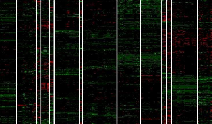
Figure 4 Results of clustering 958 high expressing ORFs over 213 conditions, with clustering both by ORF and by condition, plus high level dendrogram showing the 14 highest level condition clusters and their relationships in the clustering hierarchy. ORF clusters are not broken out or analyzed. The ORFs had defined (i.e., "non-null") estimated relative abundance values for all 213 conditions and showed evidence of induction or repression as well as high median abundance (see Supplemental Methods). ORFs are presented as lines and conditions as columns of cells, with each cell representing the log10 estimated relative abundance of the ORF in a condition, expressed in standard units for the ORF over all 213 conditions. Red values indicate negative standard unit values and therefore represent lower than average relative abundance in the condition. Green values indicate positive standard unit values and represent greater than average relative abundance. Brighter red (green) values indicate more negative (positive) abundance levels. Dendrogram branch heights and arrowheads are as in Figure 3. Cluster symbols are series codes (see Table 1) except for the following: D/msc51 = Der_diaux (D), plus four small series Der_tup, Spe_cln3, Spe_clb2, Spe_wtgal, plus the conditions Chu_spo_cont, Chu_spo_exp_0, and Chu_ndt80_del_cont (see text above for discussion). Y/Cg = Der_yap (Y) + Chu_gal_ndt80 (Cg). Spo = Chu_spo except for Chu_spo_cont and Chu_spo_exp_0 (in D/msc51 above). Spe_elut* = same as Spe_elut* in Figure 3. 60 = conditions Spe_elut_cont_60 and Spe_elut_exp_60 missing from Spe_elut* above. Spe_cdc15-1 = same as Spe_cdc15-1 in Figure 3. Spe_cdc15-2 = same as Spe_cdc15-2 in Figure 3. R = Rot. H~ts5 = all Hol non-temperature sensitive mutant conditions except for the two TAF145 wild type conditions. Hol+ts5 = all Hol temperature sensitive mutant conditions, plus the two TAF145 wild type conditions missing from Hol~ts5.

Figure 5

Figure 5 Portion of dendrogram of clustering of Figure 4 that contains diauxic shift (Der_diaux) and sporulation condition series (Chu_spo plus some small related series; see Table 1). Group g2 of the last two conditions in diauxic shift time series clusters more closely with initial / control conditions from the Chu_spo and Chu_spo_ndt80_delete series than with other diauxic shift (Der_diaux) and sporulation conditions (Chu_spo), as seen also in Figure 6b for the clustering of Figure 3. Grouping g4 contains g2 and these initial / control conditions (Chu_spo_cont_time_series, Chu_spo_exp_0, and Cho_spo_cont_ndt80_delete) but does not contain the rest of the time points from these series.

Figure 6

Figure 6 Comparison of condition clusterings of diauxic shift and sporulation time course experiment series based on microarray ratios vs. ERAs. Microarray ratios measuring changing expression profiles for yeast cells undergoing a diauxic shift employed an RNA sample from the initial time point as a control condition (DeRisi et al., 1997), and similarly for a time course measured for sporulation (Chu et al., 1998). These conditions were clustered based on log ratio data for 2467 ORFs in 79 conditions taken from (Eisen et al., 1998) and compared with clustering of the same conditions based on the ERA data clustered in Figure 3. Der_diaux, Chu_spo, and Chu_spo_ndt80_delete are series codes defined in Table 1; numbers following them indicate the hours at which an experimental samples were taken for RNA assay (except for conditions in Chu_spo_ndt80_delete where relative times are indicated). Condition designations in (Eisen et al., 1998) were relabeled in accordance with conventions used in this article. (a) Cluster dendrogram of the Der_diaux and Chu_spo conditions from the Eisen log ratio data. A 79x79 matrix of Pearson correlation coefficients of log ratio values was constructed, and the 15x79 submatrix consisting of correlations of the conditions from these series with all 79 conditions was clustered using the same clustering algorithm as Figure 3. Cluster g1 contains the initial time point from Chu_spo and the three earliest time points from Der_diaux. Cluster g2 contains the last two time points from Der_diaux. (b) Cluster dendrogram of the same series as in (a) based on ERA data described in text. A 19x217 submatrix of the 217x217 matrix of Pearson correlation coefficients employed in Figure 3 was extracted corresponding to the correlations of these conditions with all 217 conditions in the ERA file. This file was clustered as in (a). The ERA data contains 3 control conditions (containing the code "cont") and one extra Chu_spo time point compared to (a). Cluster g2 is unchanged compared to (a) but is now part of a larger cluster g3 containing initial time points from the Chu_spo and related Chu_spo_ndt80_delete series. The subtree of the full Figure 3 clustering corresponding to this dendrogram also contains conditions from several unrelated series which are not shown in this abridged clustering. (c) Illustration of potential biases in clustering of conditions based on microarray ratios over series measured with reference to different control conditions. During time course 1, cells that start in condition C₀ change progressively and end in condition C₁. During time course 2, cells start in a condition C₂ very similar to C₁ and change progressively to condition C₃. Controls for both series are initial time points indicated by *. For both time courses, ORF level ratios relative to the control condition all start near 1and change over the time course so that some ORF levels are significantly different from control condition levels and thus have ratios different from 1. Clustering algorithms applied to ratios will tend to group initial conditions such as C₀ and C₂ together based on their similar expression ratio profiles , and will not group C₁ and C₂ together based on their different profiles ( vs. ) even though these conditions are by hypothesis very similar. (d) Time course trends in microarray ratios for Chu_spo and Der_diaux. The mean square of the log ratio values in the data from (Eisen et al., 1998) is plotted for the Der_diaux ( ) and the Chu_spo ( ) time series. The abscissa represents the ordinal position of each time point in its series, not actual time. Both series begin with log ratios all near 0, corresponding to in (c), and end in conditions where some log ratios are significantly different from 1, corresponding .

References

Copyright

Copyright (c) 2000 by John Aach, Wayne Rindone, George Church and the President and Fellows of Harvard University

References

Cao, L., E. Alani, and N. Kleckner. 1990. A pathway for generation and processing of double-strand breaks during meiotic recombination in S. cerevisiae. Cell 61:1089-1101.
Cherry, J. M., C. Ball, S. Chervitz, K. Dolinski, S. Dwight, M. Harris, E. Hester, G. Juvik, A. Malekian, T. Roe, S. Weng, and D. Botstein. 1999. Saccharomyces Genome Database. http://genome-www.stanford.edu/Saccharomyces/.
Chu, S., J. DeRisi, M. Eisen, J. Mulholland, D. Botstein, P. O. Brown, and I. Herskowitz. 1998. The transcriptional program of sporulation in budding yeast. Science 282:699-705.
Chu, S., and I. Herskowitz. 1998. Gametogenesis in Yeast is Regulated by a Transcriptional Cascade Dependent on Ndt80. Molecular Cell 1:685-696.
DeRisi, J. L., V. R. Iyer, and P. O. Brown. 1997. Exploring the metabolic and genetic control of gene expression on a genomic scale. Science 278:680-686.
Eisen, M. B., P. T. Spellman, P. O. Brown, and D. Botstein. 1998. Cluster analysis and display of genome-wide expression patterns. Proc Natl Acad Sci U S A 95:14863-14868.
Everitt, B. 1980. Cluster analysis. Halsted Press, London and New York.
Marton, M. J., J. L. DeRisi, H. A. Bennett, V. R. Iyer, M. R. Meyer, C. J. Roberts, R. Stoughton, J. Burchard, D. Slade, H. Dai, D. E. Bassett, Jr., L. H. Hartwell, P. O. Brown, and S. H. Friend. 1998. Drug target validation and identification of secondary drug target effects using DNA microarrays. Nat Med 4:1293-1301.
Spellman, P. T., G. Sherlock, M. Q. Zhang, V. R. Iyer, K. Anders, M. B. Eisen, P. O. Brown, D. Botstein, and B. Futcher. 1998. Comprehensive identification of cell cycle-regulated genes of the yeast Saccharomyces cerevisiae by microarray hybridization. Mol Biol Cell 9:3273-3297.