Measuring absolute expression with microarrays using a calibrated
reference sample and an extended signal intensity range
Supplementary Material
Aimee Dudley, John Aach, Martin Steffen, George M. Church
Last modified: May 13, 2002
Contents
- Introduction
- Supplementary figures
- Supplementary tables
- Supplementary methods
- Experimental data
- Coefficient of variation analysis
- Clustering of microarray abundance vs. ratio data
- Comparison with SAGE abundances
- Scatter plots and regression sensitivity of scans of the same slide
- masliner as viewed through RI plots
- masliner software
- Abbreviations
- References
- Additional information
- Copyright
Introduction
RNA expression data collected from microarrays is usually analyzed
and presented as a set of ratios for each gene of the gene's expression
level in cells grown in an experimental condition to its expression level
in cells grown in a control condition. The ratios are derived from
scanner-measured fluorescence intensities of control and experimental
RNA or cDNA samples, each labeled with a different fluor, after
co-hybridization to a single array (DeRisi, Iyer et al. 1997).
(See Figure 1.)
While microarray-derived expression ratio data have proved invaluable to
researchers by providing sensitive and comprehensive indicators of the
molecular underpinnings of cell behaviors and states, several related
drawbacks to this form of data have been noted, including: (a) ratios
of expression levels from an experimental and control condition are
usually not convertible into absolute expression levels in the two
conditions, (b) microarray ratios involving different experimental
conditions are usually not comparable unless they are derived from
the same control condition, (c) microarray ratios are difficult to
compare with high throughput RNA expression level data derived by other
methods such as Affymetrix oligonucleotide chips
(Lockhart, Dong et al. 1996) and
SAGE (Velculescu, Zhang et al. 1995)
(see Aach, Rindone et al. 2000). Evaluation of
the statistical significance of microarray ratios has also proved
challenging, although analytical methods are improving
(Chen, Dougherty et al. 1997;
Ideker, Thorsson et al. 2000;
Kerr, Martin et al. 2000;
Roberts, Nelson et al. 2000;
Tusher, Tibshirani et al. 2001).
Use of scanner-measured intensities directly instead of ratios has been
tried as a method of addressing the fundamental comparability issues but
usually results in an unacceptable increase in error. This is because
ratios correct for several sources of bias and noise that affect intensities,
such as differences in spot size and in the efficiency
of PCR reactions used to generate the spotted probes; direct use of
intensities therefore circumvents these corrections and incurs increased
error (Aach, Rindone et al. 2000).
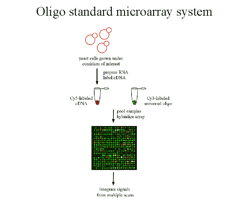
In our article we demonstrate a method for overcoming these
obstacles. First, instead of co-hybridizing labeled experimental
and control samples on an array, we co-hybridize each sample
against a standard labeled equimolar mixture of control oligos that
are complementary to microarray probes. Ratios between sample
intensities and the intensities of the oligo standards now measure
sample RNA levels on a scale that is proportional to their absolute
abundance, instead of measuring them with respect to variable and
unknown abundances of RNAs in a control sample as obtained from
the usual procedures. (See Figure 2.)
In the article we describe the advantages and
disadvantages of different kinds of equimolar standards. However,
a technical difficulty in this approach is that abundances of sample
RNAs and their corresponding equimolar controls, and likewise the
sample and control fluorescence signals measured by a scanner, can differ
by several orders of magnitude. It may therefore be difficult to
read both signals within the linear range of a scanner and derive an
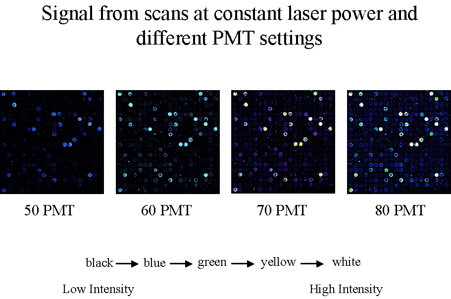
accurate measure of their ratio. Thus, as a second step in our method,
we scan each array at a series of increasing PMTGs and
use software to combine measurements from the different linear intensity
ranges corresponding to each scan into a common linear scale.
(See Figure 3.) In the
article, we describe a demonstration of this method on a dilution series
spanning a range of 1:~400,000.
In this supplementary material we make available the
masliner software used to generate a common linear scale from
multiple scans of an array, and present usage notes
and technical details relating to masliner processing.
Supplementary figures
Clicking on any of the images on the left will bring up a larger
version of the image.
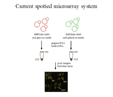 |
Figure 1 Current microarray practice involves
co-hybridizing an experimental and control sample labeled with different
fluors to the same array. Intenisities read from each fluor are transformed
into measures of ratios of expression level. Transformation to ratios corrects
for important sources of error but makes it difficult to compare expression
data across experiments. |
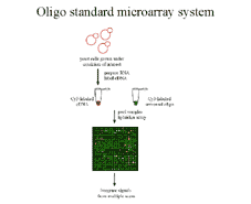 |
Figure 2 We propose co-hybridizing an
experimenal sample with a standard equimolar mixture of oligos
to the same array. Ratios of intensities now estimate absolute vs.
relative expression levels, making it easier to compare expression
data across experiments. |
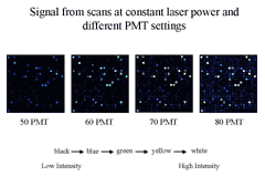 |
Figure 3 To permit accurate measurement of
intensities of equimolar controls with RNA species whose abundance
varies over several orders of magnitude, we scan an array at multiple
PMTGs and consolidate intensities of each
into a common linear scale using masliner
software.
|
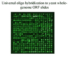 |
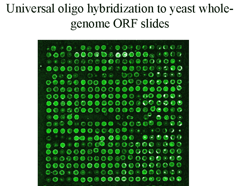
Figure 4 Scans of the equimolar control oligos
have a different appearance than conventional microarray scans because
all spots light up at approximately the same abundance.
|
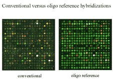 |
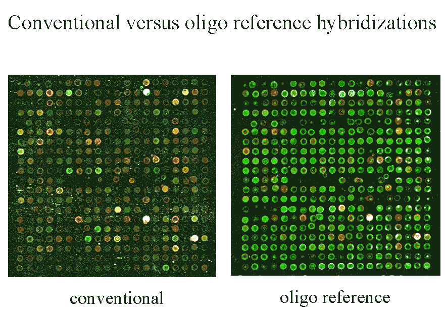
Figure 5 A direct comparison of a scan of
a conventional microarray and a scan of equimolar control oligos.
|
Supplementary tables
Supplementary table I
Processing through the masliner algorithm accurately
reconstructs abundance measurements over the range tested
(data for experiment presented in the article).
| ORFa |
Slide 1b
Cy5 |
Slide 1
Cy3 |
Slide 2
Cy5 |
Slide 2
Cy3 |
Average Ratioc |
Dilutiond |
| FBP1 |
240,452 +/- 1,998 |
2,364 +/- 28 |
155,731 +/- 4,257 |
2,187 +/- 3 |
86.5 +/- 21.6 |
N.A. |
| YIL057C |
937,566 +/- 3,934 |
16,920 +/- 28 |
692,420 +/- 6,156 |
19,136 +/- 3 |
45.8 +/- 13.6 |
1.89 |
| CYB2 |
195,604 +/- 1,930 |
21,519 +/- 28 |
214,022 +/- 4,361 |
23,805 +/- 3 |
9.04 +/- 0.07 |
5.07 |
| GAL3 |
278,301 +/- 2,064 |
130,901 +/- 3,780 |
155,210 +/- 4,256 |
70,519 +/- 3 |
2.16 +/- 0.05 |
4.18 |
| GAL10 |
75,405 +/- 1,816 |
187,927 +/- 3,826 |
81,846 +/- 157 |
141,685 +/- 3 |
0.490 +/- 0.124 |
4.41 |
| FUN34 |
57,190 +/- 169 |
390,390 +/- 4,121 |
42,646 +/- 157 |
279,828 +/- 6,681 |
0.1494 +/- 0.0042 |
3.28 |
| XBP1 |
8,913 +/- 169 |
370,515 +/- 4,084 |
9,195 +/- 157 |
338,730 +/- 6,762 |
0.0256 +/- 0.0022 |
5.84 |
| SIP18 |
2,448 +/- 169 |
316,364 +/- 3,991 |
3,442 +/- 157 |
426,860 +/- 6,912 |
0.0079 +/- 0.0002 |
3.24 |
| HXT5 |
410 +/- 169 |
371,872 +/- 4,086 |
705 +/- 157 |
332,438 +/- 6,753 |
0.0016 +/- 0.0007 |
4.9 |
| Bkg. SD |
217 |
25 |
205 |
3 |
N.A. |
N.A. |
a Oligos designed to hybridize to spots with low
expression levels (see supplementary table III below)
in the glucose cDNA hybridizations were labeled
and spiked into a hybridization reaction containing glucose cDNA
labeled with Cy3 and Cy5. Oligos labeled with Cy3 were added as
an equimolar mixture of 0.5 pmols of each oligo in the 80
 hybridization mixture. Oligos labeled
with Cy5 were added as a 5-fold dilution series in the order shown
from 100 pmols of FBP1 to 0.256 fmols of HXT5 in the 80
hybridization mixture. One standard deviation of the local background
on each slide is shown as a representation of background
fluorescence levels (Bkg. SD).
hybridization mixture. Oligos labeled
with Cy5 were added as a 5-fold dilution series in the order shown
from 100 pmols of FBP1 to 0.256 fmols of HXT5 in the 80
hybridization mixture. One standard deviation of the local background
on each slide is shown as a representation of background
fluorescence levels (Bkg. SD).
b Background-subtracted fluorescence intensities
(BSIs) +/- estimated error of prediction associated
with masliner linear regression(s) are shown for both fluors
(Cy5 and Cy3) in two repeats of the experiment (Slides 1 and 2).
BSIs and associated error estimates
were normalized by total fluorescence.
c For each slide, the Cy5:Cy3 ratio was calculated.
The average ratio +/- the standard deviation for the two repeats
is shown. N.A. stands for not applicable.
d The relative abundance values for each oligo in the
dilution series were calculated from the average ratios. Since each
Cy5-labeled oligo was added at a 5-fold lower concentration than the
previous oligo, the dilution was calculated by dividing the average
ratio of one oligo by the average ratio of the next oligo in the
series. The dynamic range of ratios detected (5.4 x 10⁴)
is the product of the dilution series; a perfect series would
produce a value of 58 or 3.9 x 10⁵.
Supplementary table II
Processing through the masliner algorithm accurately
reconstructs abundance measurements over the range tested
(an additional experiment using a different order of oligos
in the dilution series to test concentration versus sequence
specificity of Cy3 saturation).
| ORFa |
Slide 1b
Cy5 |
Slide 1
Cy3 |
Slide 2
Cy5 |
Slide 2
Cy3 |
Average Ratioc |
Actual Dilutiond |
Measured Dilution |
| GAL10 |
105,803 +/- 1,519 |
165 +/- 50 |
95,478 +/- 1,768 |
241 +/- 52 |
520 +/- 174 |
N.A. |
N.A. |
| GAL3 |
109,939 +/- 1,536 |
606 +/- 50 |
59,654 +/- 92 |
497 +/- 52 |
151 +/- 43 |
5 |
3.4 |
| CYB2 |
140,813 +/- 1,676 |
4,269 +/- 50 |
61,439 +/- 92 |
3,945 +/- 52 |
24 +/- 12 |
5 |
6.2 |
| YIL057C |
107,894 +/- 1,528 |
26,693 +/- 50 |
96,537 +/- 1,772 |
29,246 +/- 52 |
3.67 +/- 0.52 |
5 |
6.6 |
| FBP1 |
20,913 +/- 96 |
39,484 +/- 50 |
20,023 +/- 92 |
38,758 +/- 52 |
0.523 +/- 0.0092 |
5 |
7 |
| FUN34 |
2,397 +/- 96 |
64,272 +/- 50 |
1,720 +/- 92 |
61,743 +/- 52 |
0.0326 +/- 0.0067 |
25 |
16.1 |
| XBP1 |
743 +/- 96 |
65,692 +/- 50 |
409 +/- 92 |
56,412 +/- 52 |
0.0093 +/- 0.0029 |
5 |
3.5 |
| SIP18 |
108 +/- 96 |
41,260 +/- 50 |
143 +/- 92 |
19,995 +/- 52 |
0.0049 +/- 0.0032 |
5 |
1.9 |
| HXT5 |
108 +/- 96 |
36,711 +/- 50 |
220 +/- 92 |
27,218 +/- 52 |
0.0055 +/- 0.0036 |
5 |
0.88 |
| Bkg. SD |
107 |
37 |
96 |
47 |
N.A. |
N.A. |
N.A. |
a Oligos designed to hybridize to spots with low
expression levels (see supplementary table IV below)
in the glucose cDNA hybridizations were labeled
and spiked into a hybridization reaction containing glucose cDNA
labeled with Cy3 and Cy5. Oligos labeled with Cy3 were added as
an equimolar mixture of 0.5 pmols of each oligo in the 80
hybridization mixture. Oligos labeled with Cy5 were added as
a 5-fold dilution series in the order shown from 100 pmols of
GAL10 to 0.05 fmols of HXT5 in the 80
hybridization mixture. One standard deviation of the local
background on each slide is shown as a representation of background
fluorescence levels
(Bkg. SD).
b Background-subtracted fluorescence intensities
(BSIs) +/- estimated error of prediction
associated with masliner linear regression(s) are shown
for both fluors (Cy5 and Cy3) in two repeats of the experiment
(Slides 1 and 2). BSIs and associated
error estimates were normalized by total fluorescence.
c For each slide, the Cy5:Cy3 ratio was calculated.
The average ratio +/- the standard deviation for the two repeats
is shown. N.A. stands for "not applicable."
d The relative abundance values for each oligo in
the dilution series were calculated from the average ratios. The
actual dilution is the value in the dilution series that was added
to the hybridization reaction. The measured dilution is the value
in the dilution series that was measured by the scanner and adjusted
by masliner. Since each Cy5-labeled oligo was added at a 5-fold lower
concentration than the previous oligo, the dilution was calculated by
dividing the average ratio of one oligo by the average ratio of the
next oligo in the series. The 25-fold dilution between FBP1 and
FUN34 is due to a missing data point from an oligo that did not hybridize
to any of the arrays.
Supplementary table III
Background fluorescence contributed by the Cy5 and Cy3 labeled
glucose cDNA sample. In this experiment, the labeled cDNA samples
were hybridized to the oligo array without the addition of the spiked
oligos listed in supplementary Table I. This
experiment was done in parallel with the experiments presented in
supplementary Table I above. Both sets of data
were processed through masliner and normalized as described
in the article.
| |
No labeled oligos |
| ORF |
Cy5 |
Cy3 |
| FBP1 |
766 |
1,675 |
| YIL057C |
691 |
1,117 |
| CYB2 |
628 |
717 |
| GAL3 |
557 |
904 |
| GAL10 |
593 |
899 |
| FUN34 |
1,241 |
1,060 |
| XBP1 |
1,138 |
1,357 |
| SIP18 |
815 |
1,292 |
| HXT5 |
221 |
171 |
| Bkg. SD |
221 |
13 |
Supplementary table IV
Background fluorescence contributed by the Cy5 and Cy3 labeled
glucose cDNA sample. In this experiment, the labeled cDNA samples
were hybridized to the oligo array without the addition of the spiked
oligos listed in supplementary Table II. This
experiment was done in parallel with the experiments presented in
supplementary Table II above. Both sets of data
were processed through masliner and normalized as described
in the article.
| |
No labeled oligos |
| ORF |
Cy5 |
Cy3 |
| GAL10 |
125 |
46 |
| GAL3 |
91 |
46 |
| CYB2 |
91 |
46 |
| YIL057C |
101 |
46 |
| FBP1 |
91 |
46 |
| FUN34 |
91 |
182 |
| XBP1 |
101 |
46 |
| SIP18 |
1,968 |
3,244 |
| HXT5 |
91 |
46 |
| Bkg. SD |
91 |
46 |
Supplementary table V
Conventional and reconstructed microarray ratio values +/- standard errors
of the mean of these ratios for the 8 genes displayed in Figure 4 of the article.
| Gene |
Typea |
gal/glu
conventionalb |
gal/glu
reconstructedc |
gal/(gal+glu)
conventionald |
gal/(gal+glu) reconstructede |
| GAL1 |
gal |
42.14 +/- 20.11 |
84.43 +/- 41.6 |
0.939 +/- 0.034 |
0.965 +/- 0.02 |
| GAL7 |
gal |
157.05 +/- 62.92 |
155.74 +/- 60.00 |
0.989 +/- 0.004 |
0.988 +/- 0.005 |
| COX5A |
mito |
5.42 +/- 1.16 |
4.06 +/- 2.22 |
0.825 +/- 0.036 |
0.687 +/- 0.096 |
| QCR7 |
mito |
3.94 +/- 0.86 |
4.46 +/- 0.88 |
0.771 +/- 0.052 |
0.8 +/- 0.033 |
| RPL3 |
glu |
0.31 +/- 0.03 |
0.6 +/- 0.28 |
0.236 +/- 0.019 |
0.316 +/- 0.092 |
| RPL29 |
glu |
0.36 +/- 0.06 |
0.35 +/- 0.06 |
0.261 +/- 0.034 |
0.254 +/- 0.036 |
| PHO88 |
const |
0.97 +/- 0.14 |
1.45 +/- 0.76 |
0.484 +/- 0.035 |
0.474 +/- 0.117 |
| STE5 |
const |
1.02 +/- 0.24 |
3.14 +/- 2.19 |
0.485 +/- 0.057 |
0.502 +/- 0.161 |
aGenes in Figure 4 were selected to represent the following
types: "gal" = galactose-induced gene, "mito" = mitochondrial gene,
"glu" = glucose-induced gene, "const" = constitutive gene.
bAverage of four replicates of conventional microarray
ratios derived from galactose-grown experimental samples and glucose-grown
reference samples. Error is standard error of the mean of
the four replicates.
cReconstructed gal/glu ratio derived from four
gal:oligo measurements based on galactose-grown experimental
samples vs. a common oligo reference, and from four glu:oligo measurements based
on glucose-grown experimental samples vs. a common oligo reference.
Details on the derivation of these reconstructed gal/glu
ratios and their standard errors of the mean are described in
Supplemental methods below.
dAverage of four gal/(glu+gal) values +/- standard error
of the mean of these values derived from the four gal/glu values
whose average is given in the "gal/glu conventional" column
of this table. Each gal/(gal+glu) value was computed as
(gal/glu)/(1+(gal/glu)).
eReconstructed gal/(gal+glu) ratio derived from four
gal:oligo measurements based on galactose-grown experimental samples
vs. a common oligo reference, and from four glu:oligo measurements based
on glucose-grown experimental samples vs. a common oligo reference.
Details on the derivation of these reconstructed gal/(gal+glu)
ratios and their standard errors of the mean are described in
Supplemental methods below.
Supplementary table VI
This table is supplementary to Table 1 of the article. It gives a per
slide breakdown of the counts of background and saturated spots for the
two replicates whose averages were given in Table 1. These replicates
were used in the spiked oligo experiment described in the article.
To get these figures only spots corresponding to genes on the slides
were considered (6307). Standard deviations (SDs) of the median pixel
background were computed for scans performed at
PMTG 65% and 75% (Cy5), and at PMTG
75% and 85% (Cy3), for the two replicate slides E2 and F2. The columns
labeled "65_75" give statistics for the scan pair Cy5 65% and Cy3 75%,
and those labeled "75_85" for the scan pair Cy5 75% and Cy3 85%. The
masliner columns pertain to the data obtained from masliner
runs that combined four Cy5 scans and four Cy3 scans. The highest
PMTG values for these scan series were the Cy5 75%
and Cy3 85% scans; masliner background SDs are therefore the same
as for the "75_85" columns. Numbers and percents of background spots
and saturated spots are based on the 6298 of the 6307 spots for which
no oligos were spiked in. Background spots are those for which either
the Cy5 or Cy3 BSIs is < twice the background SD
measured for the fluor. For "65_75" and "75_85", saturated spots are those
for which either the Cy5 or Cy3 BSI is > 60000.
For masliner, saturated spots are those for which the
masliner-computed SATURATION-FLAG is on.
| |
65_75 |
75_85 |
masliner |
| |
E2 |
F2 |
avg +/- SD |
E2 |
F2 |
avg +/- SD |
E2 |
F2 |
avg +/- SD |
| background SD (Cy5, Cy3) |
(45,5) |
(23,0) |
|
(169,12) |
(88,1) |
|
(169,12) |
(88,1) |
|
| background spots (%) |
784 (12) |
623 (10) |
703.5+/-113.8
(11.2+/-1.8) |
648 (10) |
657 (10) |
652.5+/-6.4
(10.4+/-0.1) |
648 (10) |
657 (10) |
652.5+/-6.4
(10.4+/-0.1) |
| saturated spots (%) |
130 (2) |
62 (1) |
96+/-48.1
(1.5+/-0.8) |
294 (5) |
197 (3) |
245.5+/-68.6
(3.9+/-1.1) |
0 (0) |
0 (0) |
0+/-0
(0+/-0) |
Supplementary methods
Microarrays
Microarrays containing 6,216 PCR-amplified
yeast ORFs with a common sequence tag were produced as follows.
PCR products were re-amplified from purified PCR products corresponding
to the Yeast GenePairs products (Research Genetics). The PCR
products were re-amplified using Taq/PfuTurbo (20:1, units) with
universal forward (5'-GGAATTCCAGCTGACCACC) and reverse
(5'-GATCCCCGGGAATTGCCATG) primers for 30 cycles, annealing at
65 C and extending for 4 minutes. The
forward primer also contained 5' acrydite and amino modifications
(Operon). These modifications were introduced to facilitate binding
to alternative slide chemistries, but are not relevant for attachment
to the polylysine slides used in this study. The quality and yield of
each PCR reaction was assessed by agarose gel electrophoresis;
475 PCR reactions failed to yield a single band. The list of failed
PCR reactions is available here. PCR
products were purified by ethanol precipitation and respuspended
in 150 mM potassium phosphate (pH 8.0). PCR products were printed
onto polylysine slides (CEL Associates, Houston) using a piezoelectric
printer (Steffen, Huang, and Church, unpublished data). Slides were
UV cross-linked, washed in 0.1% SDS, and boiled in dH2O for 3 min.
ORF arrays were pre-hybridized as described previously
(Hegde, Qi et al. 1997).
C and extending for 4 minutes. The
forward primer also contained 5' acrydite and amino modifications
(Operon). These modifications were introduced to facilitate binding
to alternative slide chemistries, but are not relevant for attachment
to the polylysine slides used in this study. The quality and yield of
each PCR reaction was assessed by agarose gel electrophoresis;
475 PCR reactions failed to yield a single band. The list of failed
PCR reactions is available here. PCR
products were purified by ethanol precipitation and respuspended
in 150 mM potassium phosphate (pH 8.0). PCR products were printed
onto polylysine slides (CEL Associates, Houston) using a piezoelectric
printer (Steffen, Huang, and Church, unpublished data). Slides were
UV cross-linked, washed in 0.1% SDS, and boiled in dH2O for 3 min.
ORF arrays were pre-hybridized as described previously
(Hegde, Qi et al. 1997).
Microarrays containing the Yeast Genome Oligo Set (Operon
Technologies) were printed at a concentration of 10 pmols/ml in
150 mM potassium phosphate (pH 8.0) onto 3D-LinkTM slides (Motorola)
using an OmniGridTM microarrayer (GeneMachines). Following printing,
slides were processed according to the manufacturer's instructions.
Oligo arrays were boiled for 3 min. and shaken dry prior to
hybridization.
Both types of microarrays were hybridized and washed as follows.
Fluorescently labeled probes plus 20 mg salmon sperm DNA (Life
Technologies) and 20 mg polyadenylic acid (Sigma) were denatured at
90 C for 3 min. Pre-warmed (42 C)
hybridization buffer was added to the probe samples at a final
concentration of (25% formamide, 5X SSC, 0.1% SDS) in a final
volume of 80 ml. Hybridizations were carried out using LifterSlipTM
cover glass (Erie Scientific) and CMTTM hybridization chambers (Corning).
Hybridizations were performed at 42 C for approximately
16 hours. Slides were washed at room temperature for 5 min. with shaking
in each of the following: 0.2X SSC/0.1% SDS, 0.2X SSC, and 0.1X SSC.
Reconstructed ratio comparisons
We statistically compared reconstructed expression ratios with actual
conventional microarray ratios in two ways based on conventional
gal:glu ratios for 6297 spots derived from four independent replications
of galactose and glucose sample microarray co-hybridizations, and four
sets each of abundance levels derived from independent gal:oligo and
glu:oligo microarray hybridizations for the same 6297 spots. All
intensities in both the four conventional and 8 calibrated oligo
reference experiments were adjusted by masliner.
In our first comparison of reconstructed vs. conventional microarray
ratios, we computed 6297 two-sided t-tests for gal:glu ratios
from the four conventional microarray hybridizations against four
reconstructed ratios formed by taking the individual gal:oligo values
and dividing by the average of the four corresponding glu:oligo values.
If the distributions are equivalent, 5% of the t-tests for equality
should be rejected at P < 0.05. In fact, 346/6297 =~ 5.5% of all
t-tests were rejected, a result consistent with the hypothesis
that the reconstructed and conventional microarray ratios are statistically
equivalent. This method allowed easy computation of a standard deviation
for the reconstructed ratios by reconstructing all ratios using a
constant denominator, but may be criticized for neglecting (a) the fact that
this denominator comes from a distribution and has its own variance,
(b) the possible lack normality of the reconstructed ratio distribution,
and (c) the small number of values considered by the t-test
(four for both conventional and reconstructed ratios). t-tests were
computed in Excel 2000 (Microsoft: Seattle).
To overcome these limitations, we performed a second set of statistical
tests that compared reconstructed ratios derived from individual
gal:oligo and individual glu:oligo values (rather than average glu:oligo
values) against the four conventional gal:glu ratios using the Wilcoxon
rank sum test, which does not require any particular type of distribution.
With four values available for gal:oligo and glu:oligo each, 256 such
reconstructed ratios are possible for each of the 6297 spots, but as
the Wilcoxon test demands that all values be independent we randomly
selected 8 of the 24 possible series of four reconstructed ratios for
which each of the gal:oligo and glu:oligo values were used only once.
E.g., the first of the 8 sets of reconstructed ratios comprised the four
ratios gal:oligo(1)/glu:oligo(1), gal:oligo(3)/glu:oligo(2),
gal:oligo(2)/glu:oligo(3), and gal:oligo(4)/glu:oligo(4), where
gal:oligo(n) indicates the gal:oligo value for the nth
replicate (and similarly for glu:oligo(n)). We calculated
these 8 sets of four reconstructed ratios in the same way for each spot,
excluding from consideration 8 spots which had at least one glu:oligo
value of 0 (leaving N = 6289). For each of these 6289 spots, we performed
8 two-sided Wilcoxon tests each comparing the four conventional microarray
gal:glu ratios with one of the 8 sets of four reconstructed ratios, a total of
50312 tests, using SPLUS 6.0 (Insightful: Seattle). All p-values were
computed exactly from rank sums except for 202 which involved rank ties
(0.4%). We then found the fraction, for each of the 8 comparisons, the
fraction of tests for which P <= 0.05:
| comparison |
fraction with P<=0.05 |
| 1 |
0.0159 |
| 2 |
0.0137 |
| 3 |
0.0145 |
| 4 |
0.0084 |
| 5 |
0.0119 |
| 6 |
0.0127 |
| 7 |
0.0189 |
| 8 |
0.0107 |
In theory, for equivalent distributions, the percentage of tests
for which P<=0.05 should be ~5%. If the reconstructed and
conventional microarray ratios had different central locations, we
would expect to see fractions > 5%. Here all fractions are ~1%,
lower than expected. Part of this may be explicable by the small
numbers of values in each series. Given two series of four values, all
assumed unequal, one of the series of four can have only 70 possible
rank sums and a two-tailed test can only be rejected at P <= 0.05
at the two extreme rank sum values. Thus, the critical region for
this test actually comprises only 2/70 =~ 2.9% of the distribution.
The fact that the actual fractions are still all less than 2.9%
suggests some possible additional bias in the distributions.
Nevertheless, these results are also still consistent with hypothesis
that the reconstructed and conventional microarray ratio distributions
are equivalent.
Reconstructed ratio and standard error computations
For Figure 4 in the article, Supplemental table V (on
which Figure 4 was based), and our Coefficient of variation analysis,
reconstructed ratios were derived as follows: From four independent
masliner-adjusted gal:oligo abundance measurements for each
microarray spot and four independent glu:oligo abundance measurements for
each microarray spot, we computed averages and standard deviations for
all 24 possible sets of four gal:oligo/glu:oligo and gal:oligo/(gal:oligo+glu:oligo)
ratios, where in each set of four ratios each gal:oligo and glu:oligo
measurement was only used once. Reconstructed gal/glu and gal/(gal+glu) ratios
were computed as the average of the 24 averages, and the standard deviations of
the reconstructed gal/glu and gal/(gal+glu) ratios were computed as the
average of the 24 standard deviations. This method of estimating gal/glu
and gal/(gal+glu) ratios was used to avoid basing estimations of ratios
and errors on non-independent series of measurements; further discussion of
these issues and some alternative computations are given above in
Reconstructed ratio comparisons.
For Figure 4 in the article and its data source
Supplemental table V, errors for reconstructed ratios
are given as standard errors of the mean based on the standard deviations
given above. Since each of the 24 standard deviations is based on a set of
four values, the standard error of the mean is therefore computed as 1/2 of
the average standard deviation for each spot.
For Coefficient of variation analysis, coefficients
of variation are computed as the reconstructed standard deviation values
divided by the reconstructed ratio values (described above), and adjusted for bias as
described in Sokal and Rohlf 1995 by multiplying by
1+1/(4n). Here n = 4. This bias adjustment is also
applied to the coefficient of the conventional microarray ratios analyzed
in this section.
Click here
to download experimental data associated with this article. We have provided
all unadjusted GenePix 3.0 image analysis files and the
masliner-adjusted GenePix files that integrate all the linear
ranges for the complete series of scans performed for each array. We
have also provided a
MIAME-compliant
description of these data files.
When assessing whether a gene exhibits an increased or decreased expression
level using masliner-adjusted abundance values based on a calibrated
oligo reference, an increase in statistical error should be expected compared
to assessments based on conventional microarray ratios because assessments
based on the abundance values require an extra aggregation of error. For instance,
for a conventional (gal/glu) microarray ratio from a galactose (gal) experimental sample
against a glucose (glu) reference sample, error in the gal/glu ratio derives from
variance in both the numerator and the denominator. For the abundance comparison,
the separate gal:oligo and glu:oligo measurements derived from the experimental
samples and reference oligo are each associated with effectively the same kind of error
as the conventional gal/glu ratio, as, indeed, each of the gal:oligo and glu:oligo
measurements are essentially conventional microarray ratios except for
their use of a calibrated reference. At this level, the error profiles of
conventional ratios and masliner-derived abundance values should be approximately
the same. However, the conventional microarray ratio results in an immediate
comparison of the galactose and glucose expression levels for a gene, while
for the abundance measurements a further computation is required to set up
a statistical test for equality, e.g., we may have to compute gal:oligo-glu:oligo
and test this difference against 0, or gal:oligo/glu:oligo and test this ratio
against 1. This further computation involves an additional aggregation of error
that is not required in the conventional case.
We sought to verify the existence of this error by computing the coefficient
of variation for 6266 spots on our microarrays for both conventional and
reconstructed ratio values for galactose vs. glucose. Details on our
computation of coefficient of variation may be found here.
We performed this exercise for both gal/glu ratios, the form of conventional
microarray ratios, and for gal/(gal+glu) ratios. The rationale for considering
the latter form of ratio is that, unlike the former, it is bounded between 0 and 1
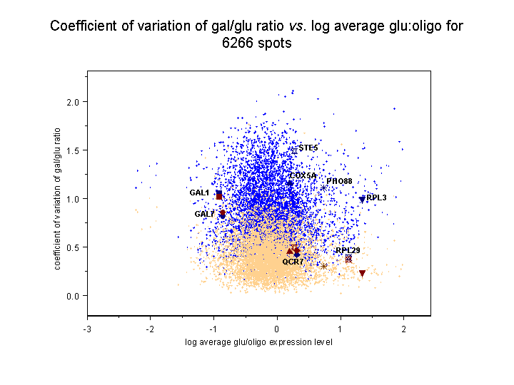
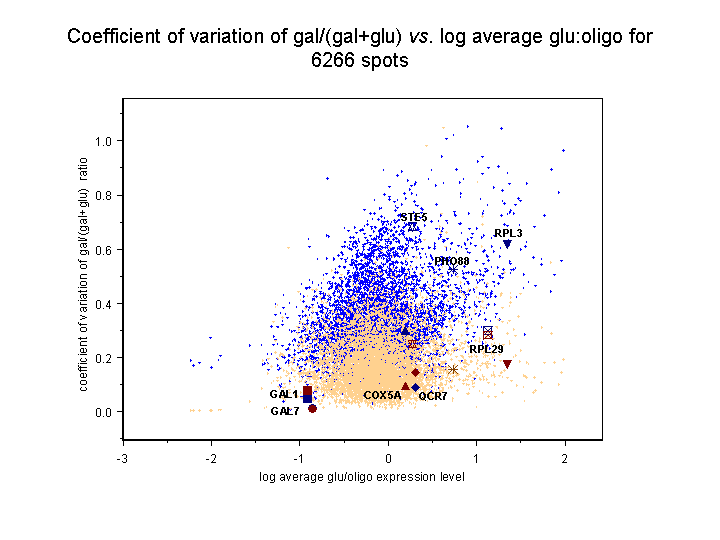
and should therefore be subject to less error overall. The results, seen below,
verify the expected increase in error for the abundance values based on
the calibrated oligo reference for both sorts of ratio.
In these images, light blue dots correspond to reconstructed ratios, and light
tan spots to dots to conventional ratios. The eight genes considered in
Figure 4 in the article text and in Supplemental table V
are highlighted with labeled spots of different shapes; the dark blue spot
for each gene corresponds to its reconstructed value and the dark red to its
conventional value. Each image is presented as a scatter plot of coefficient
of variation against the log10 average of the four glu:oligo values
for the gene, representing the degree to which the gene is expressed in glucose.
Genes that are not expressed much in glucose are therefore on the left, while
genes that are highly expressed in glucose are on the right. Clicking on either
of the thumbnail images will bring up a large version of the image.
Left panel: Coefficient of variation of gal/glu conventional and
reconstructed ratios against glucose expression level for 6256 genes.
Right panel: Coefficient of variation of gal/(gal+glu) conventional and
reconstructed ratios against glucose expression level for 6256 genes.
The average coefficient of variation +/- standard deviation for gal/glu
ratios over all 6266 spots is 0.83+/-0.38 (reconstructed) vs.
0.42+/-0.20 (conventional), while for gal/(gal+glu) ratios it is
0.33+/-0.14 (reconstructed) vs. 0.18+/-0.10 (conventional). Therefore, on
average, reconstructed ratios have a 2.0-fold higher coefficient of variation
for gal/glu values compared to conventional ratios, and a 1.8-fold higher
coefficient of variation for gal/(gal+glu) values.
Note that despite the overall increase in error for reconstructed vs.
conventional ratios, many individual genes have reconstructed errors less
than their conventional errors, including some of the genes in Figure 4 of the
article and Supplemental table 5.
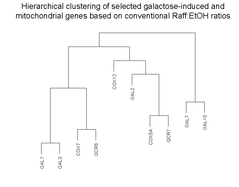
Clustering of microarray abundance vs. ratio data
In the article, we described how the loss of abundance information in
conventional microarray ratios may lead to less sensitive analysis of
differences in gene behavior compared to microarray abundance data derived
from calibrated oligo references. In particular, we showed that the
different behavior of a set of galactose-induced and a set of mitochondrial
genes could not be seen in a conventional raffinose vs. ethanol (Raff:EtOH)
microarray ratios, but can be seen in the microarray abundances derived
from raffinose vs. common oligo reference (Raff:oligo) and ethanol
vs. common oligo reference (EtOH:oligo) hybridizations. In particular,
the Raff:EtOH ratios show genes of both classes as being effectively
unchanged between the two conditions (ratios =~ 1), while the Raff:oligo
and EtOH:oligo abundances show that this is because the galactose-induced
genes are equally unexpressed in either condition, while the mitochondrial genes
are equally moderately expressed in both.
To show how the availability of abundance information affects clustering,
we clustered these 10 genes in two ways (click on thumbnails to get larger
images):
Left panel: Clustering of 10 galactose-induced and mitochondrial genes by
conventional Raff:EtOH ratios (data and genes from Table I of article).
Right panel: Clustering of these same 10 genes by Raff:oligo and
EtOH oligo (data also in Table I of article).
As can be seen, and as expected, clustering of the Raff:EtOH ratios is unable
to separate the galactose-induced genes (GAL1, GAL2, GAL3, GAL7, GAL10) from
the mitochondrial genes (COX5A, COX7, COX12, QCR6, QCR7) (see left panel),
whereas clustering of Raff:oligo and Raff:EtOH abundance values separates them
successfully (right panel). We do not take these results to indicate any
inherent limitation in clustering conventional microarray ratio data, as the
different behavior of these two sets of genes could be revealed by inclusion
into the clustering of additional sets of ratios involving other conditions
(such as galactose vs. glucose ratios). What we do suggest is that the
different behavior of these two sets of genes was already exhibited in the
two conditions examined, raffinose and ethanol, without the need for
additional conditions, but that use of conventional ratios obscured the
ability of clustering to detect it. Clustering was performed in SPLUS 6.0
(Insightful: Seattle) using Ward's algorithm
(Everitt 1980).
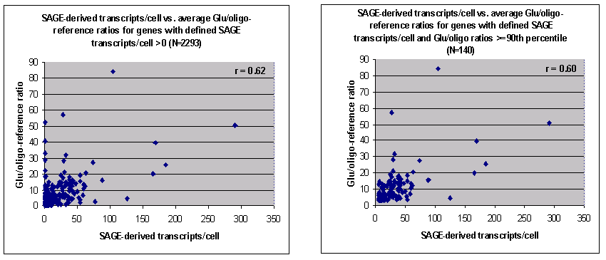
Comparison with SAGE abundances
In theory, using a universal oligo as a microarray control against
experimental samples should generate microarray ratios that are proportional
to the absolute abundances of mRNA transcripts. How close are they actually?
We attempted to address this question by comparing ratios between
masliner-adjusted ratios against universal oligo controls of
log-phase S. cerevisiae cells grown on glucose with
SAGE-derived estimates of mRNA transcript counts/cell
grown in comparable conditions (see Velculescu, Zhang et al. 1997).
To perform this comparison, we downloaded SAGE-derived
mRNA transcript counts/cell from
ExpressDB for
2442 genes for which these counts were based on unambiguous
SAGE tags (see Aach, Rindone et al. 2000)
and unambiguously associable with ORF names in our log-phase glucose
condition microarray experiments. We eliminated from this list 149 genes
whose spots on our microarray experiments failed PCR quality tests. (Go
here for a list of spots that failed PCR
quality tests.) A list of the remaining 2292 genes, their estimated
transcripts/cell from
Velculescu, Zhang et al. 1997, and the average of
their normalized masliner-adjusted intensity values in 4 microarray
hybridizations of log-phase cells grown in glucose vs. our universal oligo
standard ("Glu/oligo ratio") can be found here.
Though both the SAGE- and microarray-derived
values should estimate transcript abundances, we expect only a
moderate correlation between them because:
- Differences may exist between strain and growth conditions
between our experiments and those of
Velculescu, Zhang et al. 1997
- Despite passing PCR product quality tests, microarray measurements
for some spots may yet be of low quality if either the spot or sample
cDNAs assume secondary structures that interfere with good hybridization,
or if they contain sequences subject to high degrees of cross-hybridization.
- The different and possibly variant hybridization characteristics of
long sequences in the labeled sample to cDNA spots may not be mirrored
by the presumably more invariant behavior of the short universal oligo
control sequences to these spots.
Scatter plots of the SAGE- vs. microarray-derived
putative abundance values are shown here (click on image for larger
picture):
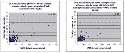
Left panel: SAGE-derived transcript abundance vs.
microarray-derived putative abundance for all 2292 genes for which both
measurements could be made. Right panel: Data for the 140 genes that
were ranked as abundant by both measures (see text below).
As can be seen, substantial scatter is evident in the
SAGE- vs. microarray-derived putative abundance values,
and the Pearson correlation coefficient between these two series is a modest
but statistically significant (see Note) 0.62.
This correlation is due mainly to genes that appear to have high
abundance in both data series (see right panel in figure above, 140 genes,
correlation = 0.60, also statistically significant -- see
Note). Genes were here considered "highly abundant"
if they had both a SAGE transcript count
and a Glu/oligo ratio >= 90th percentile in their
distributions (6 transcripts/cell and a Glu/oligo ratio of 3.01,
respectively). By contrast, the Pearson correlation between SAGE
and microarray-derived abundance values for the remaining 2152 genes
is low at 0.08 (which, however, is still significantly significant --
see Note). The difference between these
correlations is presumably due to increased Poisson
noise of genes with low SAGE tag counts and the
noise associated with genes with low microarray spot intensities.
For purposes of comparison, we also performed a correlation analysis
between SAGE-estimated transcript counts and a
set of conventional microarray ratios using these same genes. Because
absolute abundance information is lost by conventional ratios, we
expected that we would find low correlations between
SAGE and conventional ratios compared to
SAGE and common oligo reference abundances. For
the conventional ratio data set, we used the average of the glu:gal
ratios from our set of four replicates of a glucose vs.
galactose microarray experiment (the averages and their
standard deviations are reported here).
The Pearson correlation coefficient between the SAGE
transcripts/cell and the average glu:gal ratios for the entire set of 2292
genes was a surprisingly high 0.24 vs. 0.62 for the common oligo reference
correlation. This 0.24 correlation coefficient is statistically
significant compared to 0 (see Note); however
it is also statistically signficantly less than the common oligo reference
correlation of 0.62 (P < 0.0004; see Note).
The Pearson correlation coefficient for the 91 genes that had SAGE
and glu:gal ratios >= the 90th percentiles
in each series was -0.13 vs. 0.60 for the common oligo reference, indicating
that the 0.24 correlation does not reflect the genes with the strongest
signal in the two experiments. These results confirm the hypothesis that
expression levels based on a common oligo reference retain absolute abundance
information significantly better than expression levels based on conventional
microarray ratios.
As we noted in the article, we anticipate that use of equimolar
oligo reference standards (mixtures of oligos unique to each transcript
probe) will improve transcript abundance measurements by reducing the
differences between hybridization characteristics of common oligo
references and sample target sequences to the probe sequences in microarray
spots. Once such equimolar oligo reference controls are available, we
hope to repeat this comparison with SAGE or, better
yet, to perform a new comparison with SAGE or
MPSS (Brenner, Johnson, et al. 2000)
data collected on the same RNA sample assayed on a microarray using
an equimolar oligo reference standard.
The domination of correlation coefficients by the most abundant
gene products has been analyzed in another context in
Gygi, Rochon et al. (1999).
Note:
The statistical significance of the correlation coefficients
cited above was tested by generating distributions of 250 Pearson
correlation coefficients from the SAGE-derived
transcript counts against corresponding but randomly permuted microarray-derived
values. For the comparison between putative abundances
derived from common oligo reference hybridizations and
SAGE-derived transcript counts, the 0.62 correlation
of all 2292 genes and the 0.60 correlation of all 140 high abundance
genes were each > than all 250 correlations derived from the corresponding
permuted distributions. Therefore each correlation is significantly > 0
at P < 0.004. For the correlation between the remaining 2152
noise-affected genes, the actual value was > 248 of the 250 permuted
values and is therefore significantly > 0 at P < 0.012. For
the comparison between conventional gal:glu ratios and
SAGE-derived transcript counts, the 0.24 correlation
for all 2292 genes was > all 250 correlations derived from the
permuted distribution, so that P < 0.004. For the comparison between
the 0.62 and 0.24 correlations derived from the SAGE
transcript counts against the common oligo reference and conventional
microarray-derived values, respectively, a distribution of correlation
coefficients of these data series against the SAGE
data was derived from 2500 bootstrap resamplings with replacement. The
0.62 correlation from the common oligo reference was > all 2500
correlations derived from the conventional ratio data, and, likewise,
the 0.24 correlation from the conventional ratios was < than all
2500 correlations derived from the common oligo reference data. Both
results imply that the correlation from the common oligo reference
is greater than that from the conventional ratios at P < 0.0004.
The masliner strategy of integrating the linear ranges from
a series of scans of the same slide at different scanner sensitivites
relies on computation of linear regressions between the linear range
BSIs of successive scans. An example of regression-based
masliner processing is shown below. Here we discuss a number of
observations concerning the analysis of scans of the same slide including
scatter plots,
regression noise and sensitivity to outliers,
mean vs. median pixel intensity,
sublinear range bias.
 |
A single array was scanned twice on a ScanArray 5000 at constant
laser power (90%) but two PMTG settings (50% and 60%). For
each spot, the BSI from the 50% scan (s50) is plotted
against its BSI from the 60% scan (s60)
( , , , , ).
Six spots are saturated in s60 that were not saturated in s50 ().
Using masliner, a linear regression was computed for the 176 s50 vs.
s60 values within the linear range of the scanner (,
2,000 <= BSI <= 60,000). The regression was used to extrapolate
values for the six s60 saturated spots ( ).
Six spots are saturated in s60 that were not saturated in s50 ().
Using masliner, a linear regression was computed for the 176 s50 vs.
s60 values within the linear range of the scanner (,
2,000 <= BSI <= 60,000). The regression was used to extrapolate
values for the six s60 saturated spots ( ), effectively
generating an extended common linear scale for spots over both scans.
One spot saturated in s50 ( ), effectively
generating an extended common linear scale for spots over both scans.
One spot saturated in s50 ( ) had been extrapolated
to a common linear scale with s50 through an earlier scan (45%) and masliner
processing. This spot was carried into a common linear scale by masliner
processing of s50 and s60 ( ) had been extrapolated
to a common linear scale with s50 through an earlier scan (45%) and masliner
processing. This spot was carried into a common linear scale by masliner
processing of s50 and s60 ( ). Some spots
(N=6,185) were below the linear range in all three of these scans ().
3,288 of these spots were brought into the common linear scale
by additional scans at higher gains and executions of masliner. A series
of masliner adjustments using data from 4 scans increased the
intensity of the brightest spot on this array from 65,535 (saturation)
to 3.2 million units with a 0.4% estimated error associated
with the linear regression. This data was taken from the Glu:oligo
experiment presented in Table 2 of the article. Figure 1 of the article
is a slightly-edited version of this figure in which data for the spot
saturated in s50 (,)
was removed and axes scales and legends were changed.
(Click on image for larger view.) ). Some spots
(N=6,185) were below the linear range in all three of these scans ().
3,288 of these spots were brought into the common linear scale
by additional scans at higher gains and executions of masliner. A series
of masliner adjustments using data from 4 scans increased the
intensity of the brightest spot on this array from 65,535 (saturation)
to 3.2 million units with a 0.4% estimated error associated
with the linear regression. This data was taken from the Glu:oligo
experiment presented in Table 2 of the article. Figure 1 of the article
is a slightly-edited version of this figure in which data for the spot
saturated in s50 (,)
was removed and axes scales and legends were changed.
(Click on image for larger view.)
|
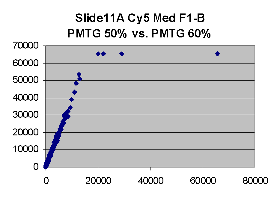
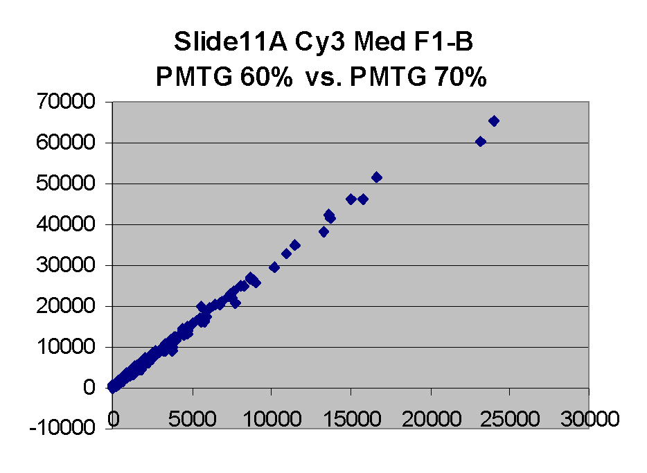
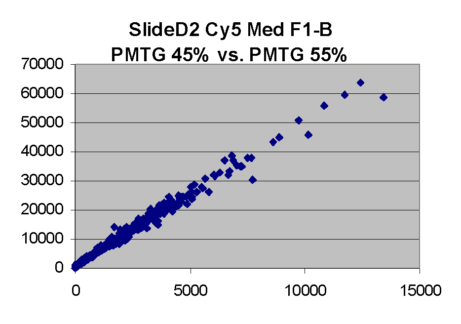
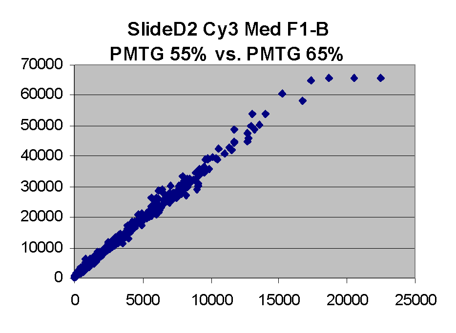
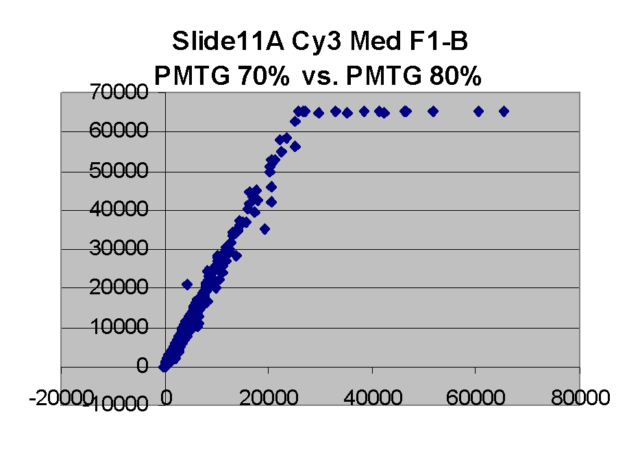
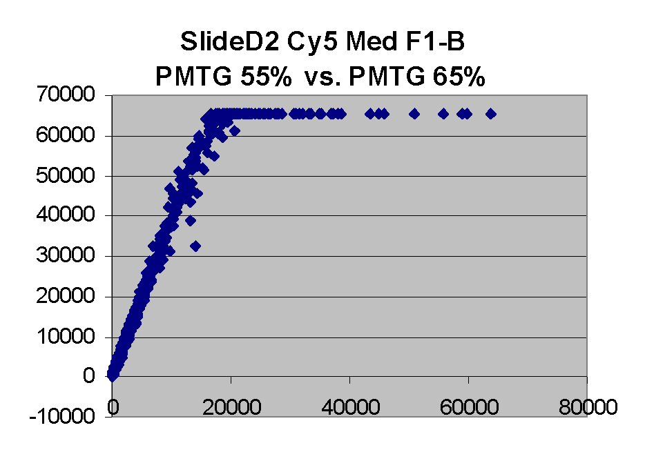
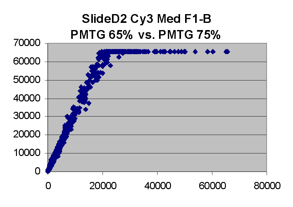
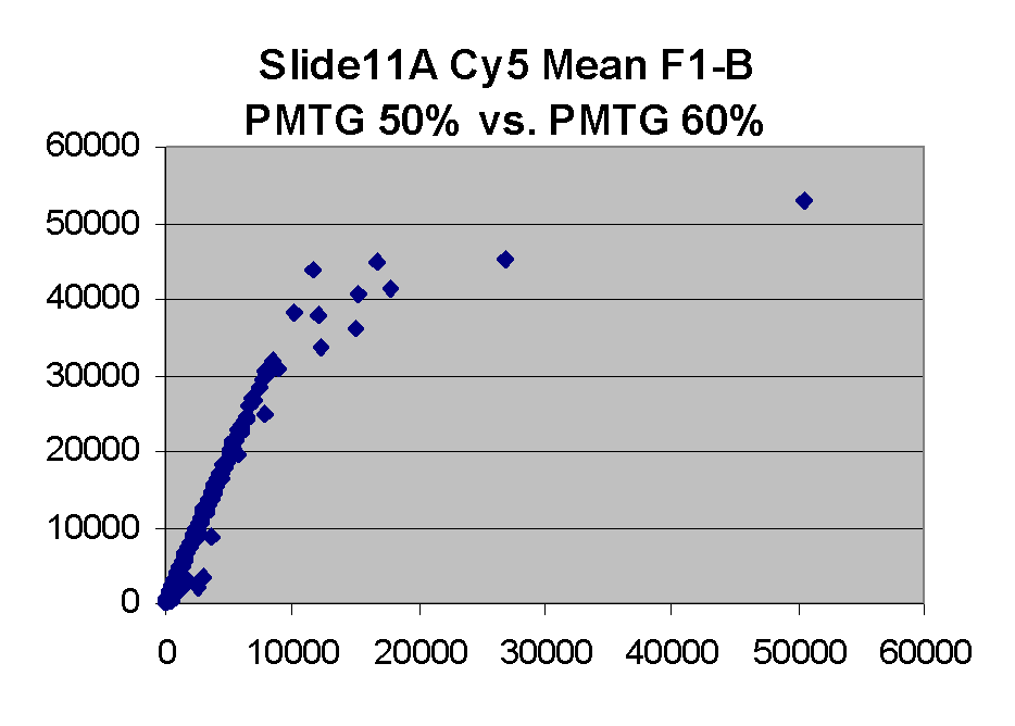
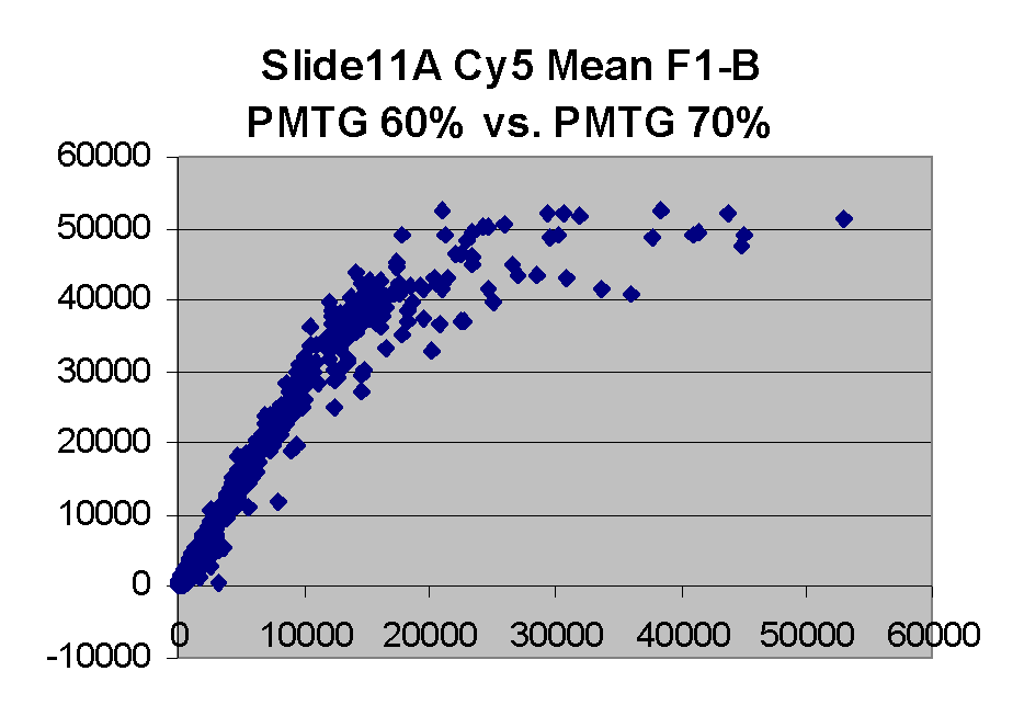
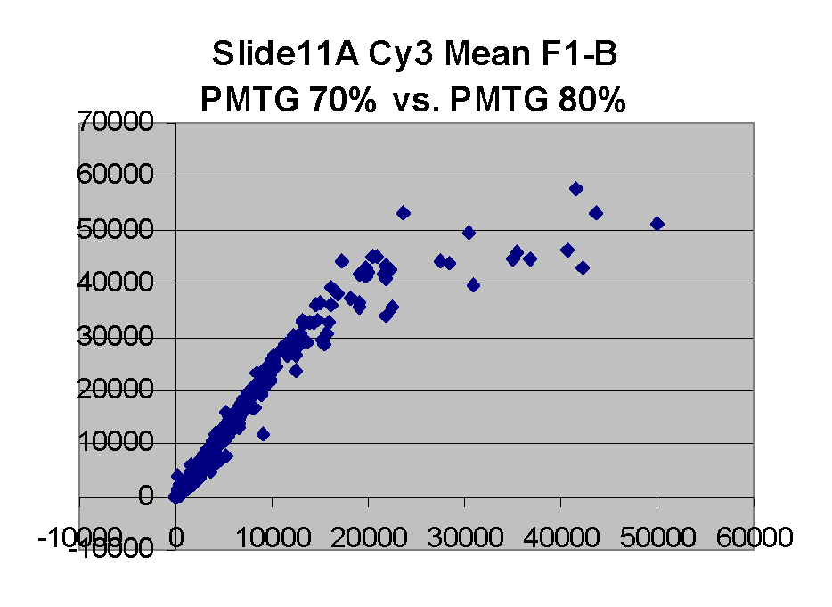
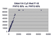
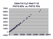
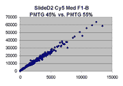
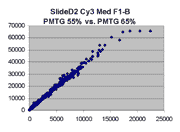
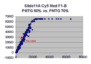
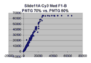
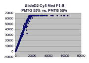
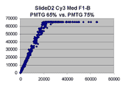
Scatter plots of scans of the same array
Below are scatter plots of linear range BSIs from
one scan against the next higher PMTG scan for
the same slide. Spots were considered to be in the linear range if
their BSIs were between 2000 and 60000 inclusive.
Here BSI measurements are given by median pixel intensity
minus background as given in GenePix 3.0 output (as used by masliner).
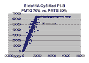
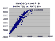
The figures on the left (Slide 11A) are from a PCR-product spotted
microarray in which the Cy5-labeled sample was yeast grown in glucose
and the Cy3-labeled sample was yeast grown in raffinose. The figures
on the right (Slide D2) are from an Operon yeast oligo spotted microarray
in which both the Cy5- and the Cy3-labled samples were yeast grown
in glucose. Both Cy5 and Cy3 images are given for each slide.
In general we find that scatter appears to increase as BSI
increases within each scatter plot, and also that more scatter appears at higher
PMTGs. This makes sense if noise is amplified along
with signal as amplification gain increases. Clicking on any image
will bring up a larger version.
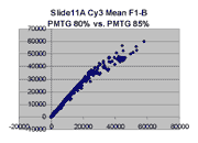
| Slide 11A |
|
Slide D2 |
| Cy5 |
Cy3 |
|
Cy5 |
Cy3 |
 |
 |
|
 |
 |
 |
 |
|
 |
 |
 |
 |
|
 |
 |
Regression noise and sensitivity to outliers
Along with noise, outliers also appear in these scatter plots.
We considered outliers from the several related perspectives: (a) the degree
to which outliers may have affected masliner regressions, and also outlier
bias, (b) whether outliers are associated with any specific causes such
as spot morphology. Regarding outlier bias in (a), visually
it appears that outliers tend to lie to the right of the dense linear body
of points approximated by the regression in each graph.
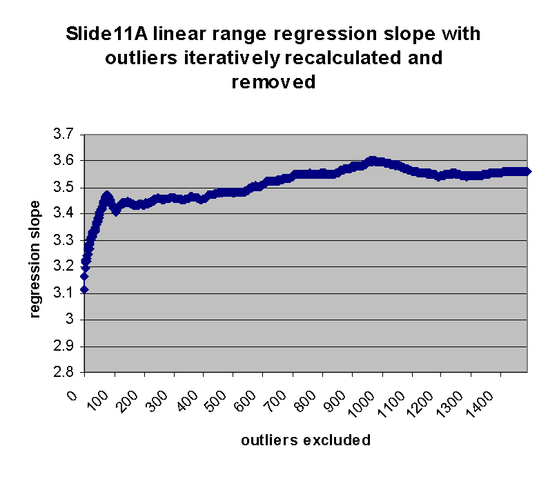
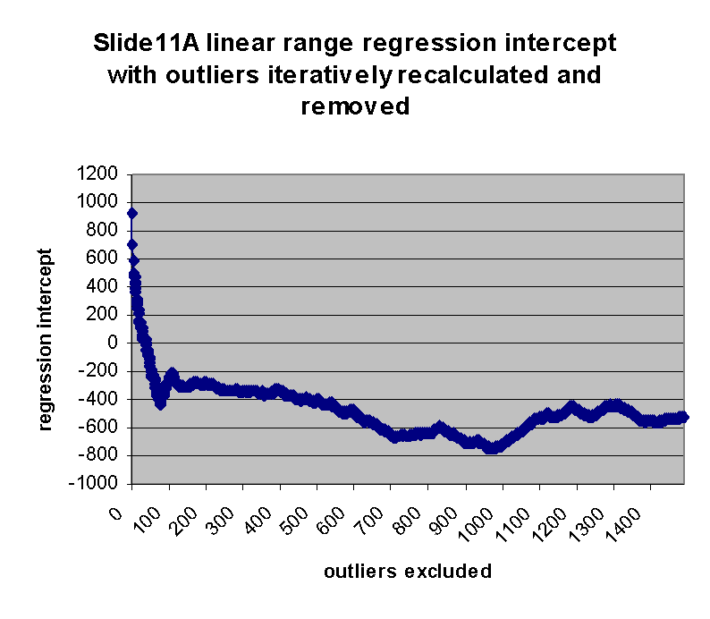
(a) Impact of outliers, outlier bias: We took the Cy5 data from the 1492 spots
corresponding to genes in the linear range of the Slide 11A scans at
PMTG 70 and 85 (lower left scatter plot above) and
performed the following computations: We computed the linear regression
of the PMTG 80 values (Yi) against
the 70 values (Xi), yielding a computed slope
m(0) and intercept b(0) such that the sum of squares of residuals
ri = (Yi - (m(0)*Xi + b(0)))
was minimized. We then removed the spot from the series with the largest
abs(ri), representing the largest outlier,
and performed a new regression, yielding a new slope m(1) and
intercept b(1). By similarly iteratively removing the largest outlier,
we obtained a series of slopes m(j) and intercepts b(j)
for j = 0,1,...,1491. The chart below shows the result:
| Regression slope |
Regression intercept |
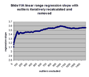 |
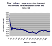 |
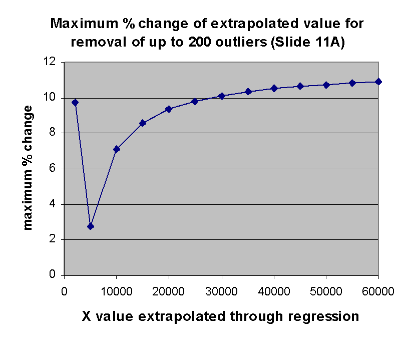
As can be seen, the regression slope curve increases from a minimum
value of ~3.11 at 0 outliers to a local peak. The location of this peak
is ~3.48 at 75 outliers removed. Regression slope then drops and tends
to rise slowly as additional outliers are removed. Similarly, regression
intercept drops from an initial maximum of ~928 to a local minimum of -433 at
75 outliers removed, and then begins to rise. The initial sharp rise in
regression slope and increase of regression intercept appears to confirm
the visual observation that outliers are biased to the right of the main
body of points, as outliers to the right tend to drag down the slope and
raise the intercept. This is also seen by the direct observation that
13 or the first 20 outliers in the first regression (resulting in
m(0) and b(0)) have negative residuals (their points therefore
lie to the right of the main body of points).
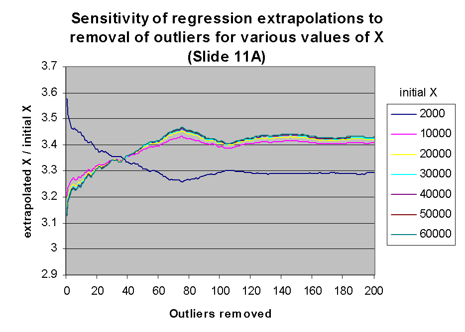
However, the degree of influence of outlier removal on slope and intercept
is modest. As currently designed, masliner performs no outlier removal
and therefore it computes adjustments based on the slope and intercept for
the complete set of points (outliers removed = 0). Assuming that outlier
removal could be reasonably limited to removal of outliers among the
first 200 points (13.4% of the 1492 points), the slope used by masliner
is a maximum of ~12% too small (100*(3.48-3.11)/3.11). Similarly, the
intercept used by masliner is at most 1361 too large (928-(-433)). As
masliner's extrapolation
m(0)*Xi + b(0) is performed mainly on
larger Xi values (as adjustments are extrapolated only for spots
that saturate in the next highest PMTG scan), the impact of
the high intercept value used by masliner is likely to be small
compared to the impact of the small slope value, so we would expect the presence of
outliers on masliner to be about 12%.
These expectations are confirmed by the following two graphs. The graph at
the left shows the value of m(j)*X + b(j) for
j between 0 and 200, for various values of X within the linear range.
The ordinate of this graph is given as the ratio of the extrapolated X to
the initial X (see graph legend), rather than extrapolated X alone,
in order to accommodate differences of scales of the extrapolated X. It
is clear that the effect of regression outliers is the same for all values of
X except the very lowest values. This behavior is explained by the
fact that only for low X values does the regression intercept have a
significant impact on extrapolation, as described above. The graph at the
right shows the maximum impact of outlier removal on extrapolation for each
of the X values exhibited in the graph at the left. The ordinate of
this graph is the maximum possible percent change in the extrapolation from X
over all the regressions involving removal of j outliers from
j = 0,1,...,200. The maximum possible percent change is
100*(max(m(j)*X+b(j))-min(m(j)*X+b(j))/min(m(j)*X+b(j))
where each max and min is over this range of j. As can be seen,
this maximum possible effect is ~ 11%, as anticipated.
As masliner is run iteratively over a series of scans, a larger
cumulative effect should be expected. E.g., if masliner-adjusted values
are 10% low, and masliner is run 3 times, than BSIs
that were adjusted 3 times would be approximately 0.93 =~ 73% what
they should be, while BSIs that were adjusted twice would
be approximately 80% of what they should be, etc.
The conclusion which we have drawn from this analysis is that regression
outliers do affect masliner adjustments, but that their impact appears
to be modest. We plan to keep an eye on this effect and will consider
implementation of outlier elimination or robust regression logic in
masliner as we gather experience with it.
(b) Causes of regression outliers: To understand the possible causes
of regression outliers, we selected a number of outliers and non-outliers from
Slide 11A and Slide D2 scatter plots and examined the images of the spots
using GenePix 3.0. We thought it possible that regression outliers might be
associable with irregular spot morphologies. However, when we examined these
spots, we found no clear indication that the spot morphologies of outlier spots
were different from those of non-outliers. One outlier spot did happen to be
a spot that had been marked as an error, but the error concerned the fact
that the spot was on the edge of a grid that overlapped another grid; the
spots on these overlapping grids did not themselves overlap and appeared to have
morphology common to normal spots.
As noted above, outliers appear to be biased towards the right.
An outlier to the right of the main body of points in a regression has a
BSI in a lower PMTG scan that is too
high, compared with most spots, than its BSI in the
next highest PMTG scan. This could either be due to (i)
pixels in the 'low' scan being too bright compared to the 'high' scan, or (ii)
pixels in the 'high' scan being too dim compared to the 'low' scan. On suggestion
of Jean O'Malley of Oregon Public Health and Sciences Universally
(and whom we gratefully acknowledge with thanks for this suggestion), we explored
whether pixel saturation in the 'high' scan could be a cause of (ii).
Examination of pixel plots in GenePix 3.0 for selected spots did reveal
that some 'high' scan pixels do appear to saturate, but we do not believe
that this leads to (ii) because we have measured BSI
by median pixel intensity minus background: For pixel saturation to
artifactually lower BSI measured by the median would
require over 50% of the pixels to become saturated, which we did not observe, and
the result would be that the 'high' scan BSI would be
saturated and therefore not in the linear range. However, the effect of
pixel saturation appears to be visible when BSIs are
measured by the mean pixel intensity minus background, as seen
below.
Finally, we also note that we have found one case of outliers which appear
to be so because they appear to be abnormally bright on a lower
PMTG scan (therefore instances of situation (i) above),
rather than because they are artifactually dim on the higher PMTG
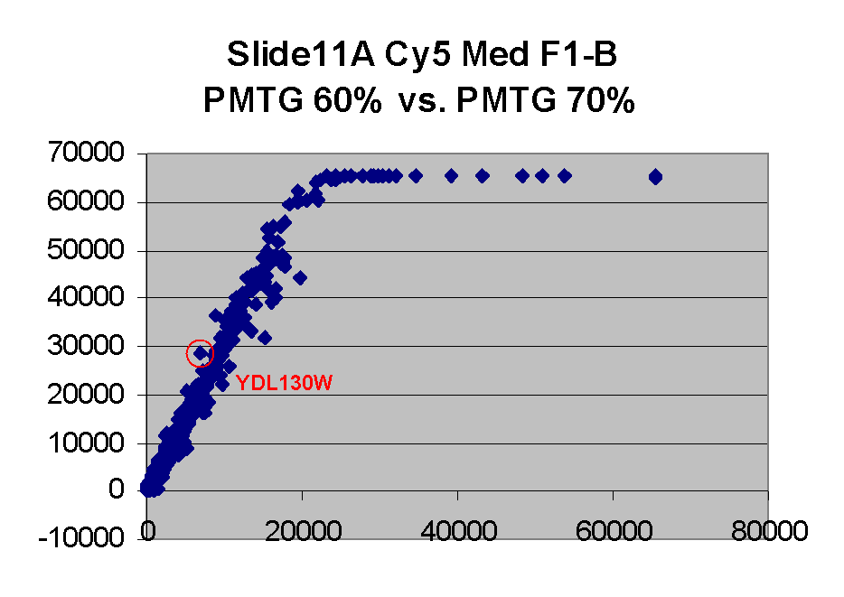
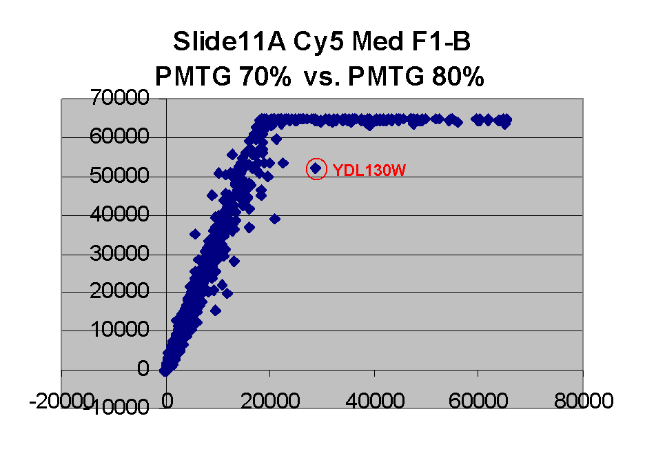
scan: In particular, the point for gene YDL130W appears to be an outlier on
the left in the Cy5 scatter plot for Slide 11 for PMTG 60% vs.
PMTG 70%, and an outlier on the right in the
Cy5 scatter plot for Slide 11 for PMTG 75% vs.
PMTG 80% (lowest two scatter plots on
the left edge above). This suggests that this spot was artifactually
bright in the PMTG 70% scan.
We conclude by noting that at this point, based on the preliminary observations
above, we do not have a hypothesis as to any mechanisms that may be associated
with regression outliers. However, it does appear that there can be considerable
scanner-based noise in BSI measurements, and one interesting
but yet unperformed experiment would be to rescan a slide at the same PMTG
and laser power to see if the same spots were found to be outliers in multiple scans.
To the extent that the presence of scanner-based noise is confirmed, we foresee another
potential advantage in the masliner strategy: the use of the multiple scans
to estimate scanner noise in BSI measurements for each spot.
Mean vs. median pixel intensity
As noted above, pixel saturation does not
appear to explain the bias of regression outliers to the right. However,
the effect of pixel saturation appears clearly visible when BSIs
are measured by the mean pixel intensity minus background, as seen
in the following Cy5 and Cy5 scatter plots for BSIs measured
by mean pixel intensity for Slide 11A. Note that there appears to be
a curvilinear distortion in the main body of points in these scatter plots
compared to their median pixel intensity counterparts (here).
Such a curvilinear distortion would be accounted for by pixel saturation in
the 'high' scan, which would tend to lower the mean pixel intensity for
points to the right in the graph. By contrast, the in median pixel intensity
plots, the main body of points appears to lie along a straight line until
saturation (although some curving appears in the highest PMTG
scatter plot for Slide D2 Cy3).
This observation supports our use of BSIs based
on median pixel intensity by masliner.
| Slide 11A Cy5 Mean-based BSIs |
Slide 11A Cy3 Mean-based BSIs |
 |
 |
 |
 |
 |
 |
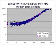
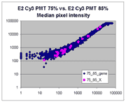
Sublinear range bias
On examining the scatter plots above, one might think that the linear
range of a scanner is bounded only above by saturation, and that there is no
reason for masliner to operate with a linear range that is also bounded
from below. However, the presence of curvilinear bias in the low range of
acquired intensities is clearly visible in scatter plots of log intensities
(log-log scatter plots). Below is shown a set of log-log scatter plots for
slide E2 for both Cy3 and Cy5, one of the slides used in the spiked oligo
experiment described in our article. These plots are based on median pixel
intensities and not background-subtracted intensities (BSIs)
of spots in the arrays to show that the curvilinear bias is not caused by
background subtraction itself. (Log-log scatter plots based on
BSIs look very similar.) Also, this spotted oligo-based
array contains many empty feature positions that are not spotted with DNA oligos for
gene products. The plots below show these positions in light blue vs. the
dark blue used for gene-based spots. Dots on the scatter plot for these
empty positions are intermixed along with the dots for gene spots, thereby
showing that the curvilinear effect comes about wholly through operation of the
scanner itself and is not dependent on the contents of the spots on the array.
The presence of this curvilinear bias justifies the need to specify and use
a lower linear range by masliner. Note that any feature
for which the Cy5 or Cy3 median pixel intensity <= 0 does not appear
on the scatter plots.
| Slide E2 Cy5 Median feature intensities |
Slide E2 Cy3 Median feature intensities |
 |
 |
 |
 |
 |
 |
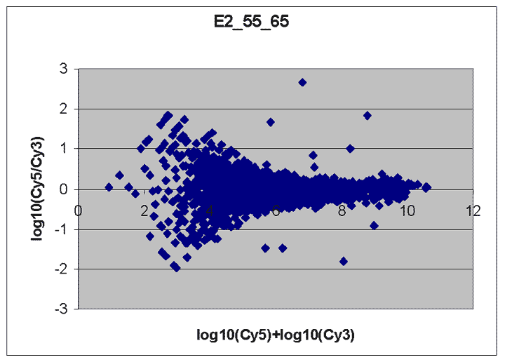
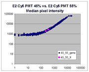
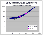
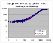
masliner as viewed through RI plots
An interesting way to view masliner operation is through
RI plots (Quackenbush, J. 2002; essentially
the same as MA plots (Yang, Y.H., Dudoit, S., et. al. 2002)).
These are plots of log(Cy5 BSI)-log(Cy3 BSI)
against log(Cy5 BSI)+log(Cy3 BSI) over all
spots on an array. Shown below are four scatter plots of slide E2, one based on
masliner-adjusted data and the other three on pairs of single Cy5 and Cy3
scans of the slide. Slide E2 is one of the arrays used in the spiked oligo
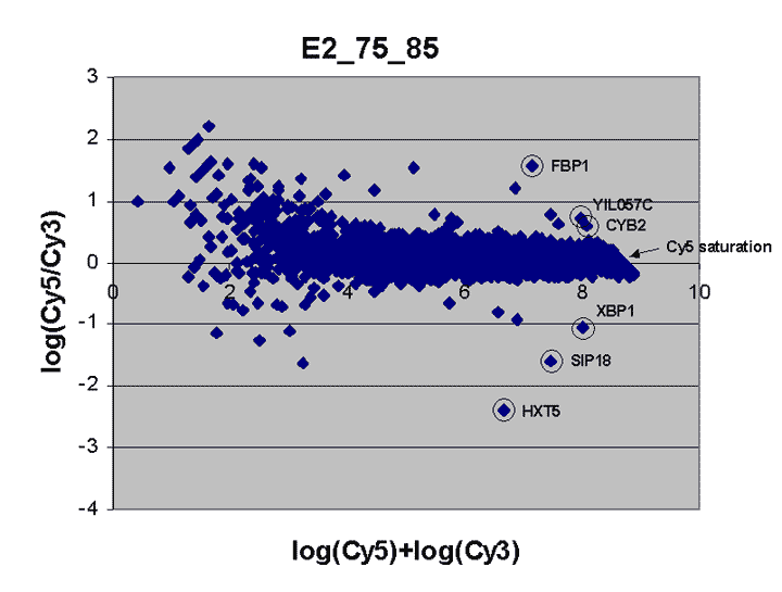
experiment described in our article. The hybridization mixture for slide E2 is a
self-self hybridization (Cy5-glucose vs. Cy3-glucose) to which a 5-fold dilution series of
Cy5-labeled oligos and an equimolar mixture of corresponding Cy3-labeled
oligos hybridizing to 9 spots were added (see article). For all other spots
Cy5/Cy3 ratios are close to 1 while, for these spots, all ratios but one differ
widely from 1 (for ratios based on slide E2 and replicate F2, see
supplementary Table I). Thus, spots associated
with spiked oligos tend to appear as outliers in these RI plots.
As described in the article, masliner-adjusted data for
this experiment has comparable or better accuracy, consistency, and
completeness compared to data derived from individual scan pairs. The plots below show
how masliner extends the signal range for the arrays, avoids saturation,
and exploits different scans for the accurate measurement of each spot.
To prepare these plots, only array features for which both the Cy5 and Cy3
BSIs were > 0 were used. Cy5 and Cy3
BSIs were then both total-normalized to 20000000.
Clicking on an image displays a larger version.
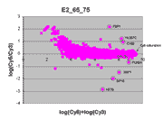 |
This RI plot is based
on a single Cy5 scan at PMTG 65% and a single Cy3 scan
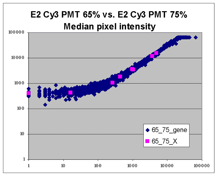
at PMTG 75%. As described in the article, data
obtained from these scans were closest in accuracy to corresponding
masliner-adjusted data. Eight of the 9 spots targeted by
spiked oligos can be identified in the plot. The sharp diagonal
edge at the right of the plot corresponds to spots saturated in the Cy5
scan.
|
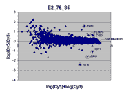 |
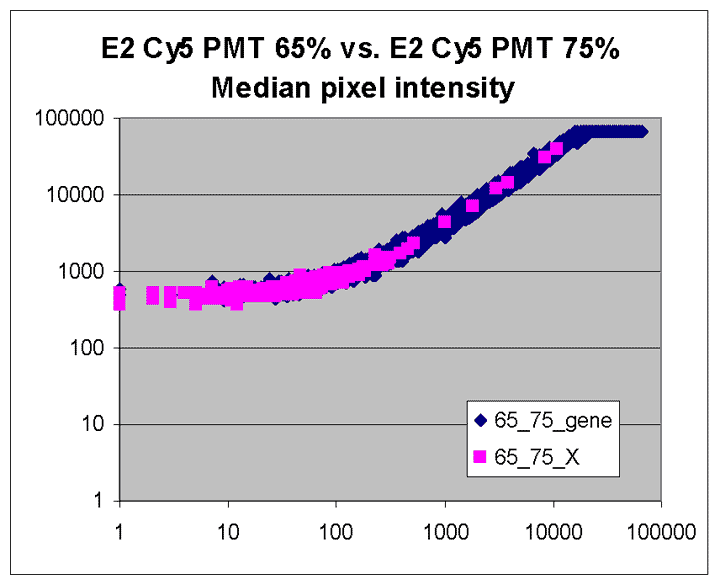
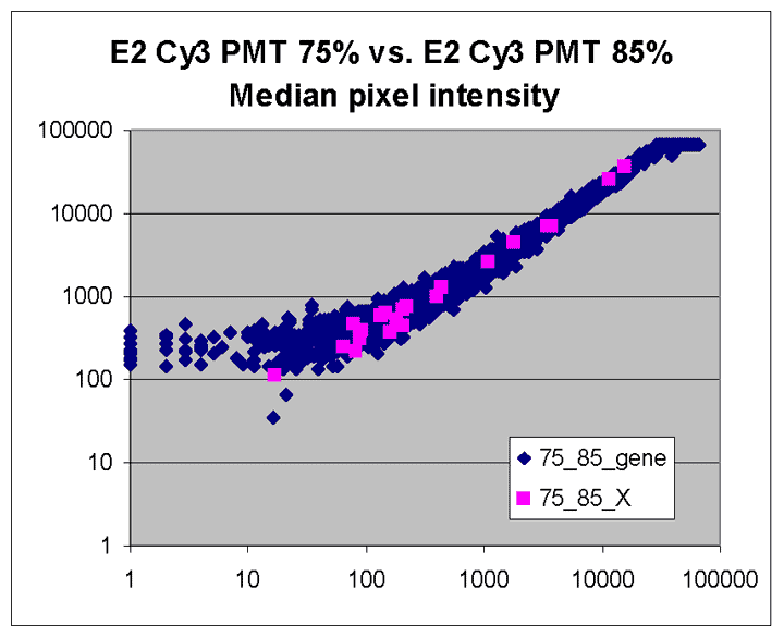
This RI plot is based
on a single Cy5 scan at PMTG 75% and a single Cy3 scan
at PMTG 85%. As described in the article, data
obtained from these scans were less accurate, consistent, and comprehensive
than the corresponding masliner-adjusted data. By virtue of the higher scan
PMTG settings compared to those for the plot above, more
spots are raised above background levels than above (see article).
Here, six of the 9 spots targeted by spiked oligos can be identified in the plot.
A larger sharp diagonal edge at the right indicates that more spots saturated
in this plot compared to above.
|
 |
This RI plot is based
on masliner-adjusted scan series of four Cy5 and Cy3 scans, including
the scans used above. Dots in the RI plot corresponding to array
features are represented by different colored symbols depending on which
Cy5 and Cy3 scans were used by masliner to pick up BSIs
for the features; since these depend on spot brightness in the two channels,
the result is that the RI plot is broken up into different regions.
For instance, the region with legend "75_85" comprises array features
picked up in the Cy5 75% and Cy3 85% scans; other legends are interpreted
similarly. The "75_85" region uses the same scans that were processed
as a pair above and are represented by the same symbol as in that RI plot;
similarly, the "65_75" region uses the same symbol as used for the Cy5 65%
and Cy3 75% pair above. The "75_85" region represents the great number
of dim spots on the array whose BSI values were
picked up by these highest PMTG scans.
The masliner plot does not exhibit the
saturation noted for the individual scan pairs above (i.e., there is no
downward diagonal edge at the right). Instead, the different colors to
the right show how saturation has been corrected by incorporation of other
scans. The masliner plot also extends to an ordinate of > 10.5 compared
to ~9.5 for the individual scan pairs due to the extended signal range
computed by masliner. The different symbols for the 8 spots
corresponding to the spiked oligos shows how masliner has leveraged
different scans towards the accurate computation of these features, whose
Cy5 and Cy3 values may differ by orders of magnitude.
|
 |
This RI plot is based
on a pair of lower intensity Cy5 and Cy3 scans. Because some Cy5 or Cy3
values were measured with a BSI = 0, some spiked oligo
features do not appear on the plot. The main reason we have included
this plot is to indicate that not all RI plots show the upward
curve to the left, and that masliner's correction for saturation
and construction of a common extended signal range does not correct for
this effect. The cause of this upward curving is unknown but
may be related to higher background levels on brighter scans. While
the masliner plot appears to have less upward curvature to the
left than the plot for scan pair Cy5 65% and Cy3 75% above, this is
only because masliner points at the left of the masliner plot
came from higher power Cy5 75% and Cy3 85% scans that exhibited
this effect to a lesser degree.
|
masliner software
masliner stands for MicroArray Spot LINEr Regression.
Obtaining the software
Go here
to obtain a copy of the masliner program.
Citing the software
Please cite usage of masliner with
Dudley, A., Aach, J., Steffen, M., and Church, G.M. (2002) Measuring absolute
expression with microarrays using a calibrated reference sample and an
extended signal intensity range, Proc Natl Acad Sci USA
99(11): 7554-7559
Usage notes
Basic help messages describing parameters may be obtained by executing
masliner without any parameters. This section provides a general
orientation to masliner use.
General orientation: masliner operates on a pair of GenePix scan analysis files
that represent scans at different PMTGs of the same
array. The files must be in the same format and describe the same spots
in the same order. The two files are specified by the -g1 and -g2 parameters.
In general, masliner parameters that relate to the input files come in
pairs with a common prefix and a suffix that is either 1 or 2.
Each of the GenePix scan files indicated by -g1 and -g2 contains columns
for measurements and calculations reported by the GenePix software.
These include measurements of mean and median pixel intensity,
background levels, and others. Each execution of masliner operates on a single
fluor from each file. To process both fluors therefore requires two executions
of masliner each of which produces an output file containing
adjusted BSIs for a single fluor.
When processing two GenePix files for a single fluor, masliner
works with the columns for median pixel intensity and median background
intensity. Median pixel intensity is given in a column whose header
begins with "Median F", and median background intensity in a column whose
header begins with "Median B". The suffixes vary from scanner to scanner
and also on GenePix options. For the GSI Lumonics ScanArray 5000 and
GenePix options used in our study, the suffixes corresponding to the two
fluors were simply "1" and "2", so that the column headings masliner
examined were "Median F1" and "Median B1" for fluor "1", and "Median F2" and
"Median B2" for fluor "2". For a collaborating group testing masliner using
an Axon scanner and other GenePix options, the column heading suffixes for
the median pixel intensity and background intensity for the two fluors were
"635" and "532", so that their GenePix files contained the columns
"Median F635" and "Median B635" (and similarly for 532). To run masliner
properly it is necessary to determine what column heading suffixes are used in
the GenePix output files for the options and fluor you wish to process, and
feed it to masliner via the "-f1" and "-f2" parameters. Here "-f1"
is the fluor specification for the "-g1" input file and "-f2" the fluor
specification for the "-g2" input file. The default value for these fields
is simply "1" (suitable for the "Median F1" and "Median B1" columns that were
generated for the files we generated). Thus, a sample command for processing
a file using the Axon scanner and GenePix parameters that our collaborators
used would begin:
masliner -g1 input1.gpr -g2 input2.gpr -f1 635 -f2 635 ... (for fluor 635)
masliner -g1 input1.gpr -g2 input2.gpr -f1 532 -f2 532 ... (for fluor 532)
Regression modes: As described in the article, masliner adjusts intensity
values in the file that corresponds to the higher PMTG
that appear to be affected by signal saturation. Adjustments are based on
linear regressions of intensities of the higher and
lower PMTG scans which are both within the
linear range of the scanner. To perform these regressions, masliner must be
told or determine the linear range of the scanner. There are
two options, selectable by means of the -m (mode) parameter.
- 'straight' mode: Here masliner is provided the linear
range of the scanner by means of the -ll (linear low) and -lh (linear
high) parameters, and uses these values as given. 'Straight' mode is
appropriate when the scanner has a well defined linear range which
you know ahead of time. We found that our scanner was strongly
linear in a range of about 2000 to 60000, above which values sharply
saturated. Defaults are set at these values.
- 'dynopt' mode: This mode is provided for situations where you
know a subrange in which the scanner is linear, but for which there
is no sharp threshold above or below which scanner response departs
from linear. Here, -ll and -lh are used to provide the subrange, and
two other parameters must be provided that instruct masliner
on how to search for the larger range. The first is -inc, which defines
increments to -ll and -lh which masliner will explore. The
second is -q, a threshold for a quality measure which is used to assure
that the quality of the linear regression in an intensity range is held
within acceptable bounds. The quality measure is defined as the
unexplained error of regression over the mean intensity of the regressed
variables (see Technical notes); therefore lower
values of the quality measure indicate better regressions. For most
of our work, we found a -q threshold of .05 produced good results.
For instance, if you know that your scanner is linear between 4000 and
30000, but its departures from linearity are not sharp but increase
continually above that range, you might use 'dynopt' mode with -ll 4000,
-lh 30000, -inc 1000 and -q .05. masliner will compute all
regressions in ranges expanded by integral numbers of -inc from the
specified -ll and -lh, e.g., masliner will consider all ranges
of the form 3000-n*1000 to 30000+m*1000, where n,m
= 0,1,2..., and increments stop when a range contains the data maximum or minimum.
The n and m for which the expanded range is the largest and for which
the regression quality >=.05 will be chosen as the optimum linear range,
and the regression computed on that range will be used to adjust values
in the higher PMTG scan.
Output file: masliner output consists of an adjusted copy of the higher
PMTG input file. All adjustments are made in a set of four
extra columns for each spot at the end of columns copied from the input file.
- ADJCOUNT gives the number of times a spot value has been adjusted and is
0 if the spot's value has never been adjusted.
- ADJBSI contains the adjusted BSI value computed for
a spot, calculated from the masliner-determined regression on the
lower PMTG scan BSI value. If the
spot has not been adjusted (i.e., ADJCOUNT is 0), ADJBSI contains the
higher PMTG scan's BSI value and
will thus be equal to the value F1 Median minus B1 Median (for fluor 1) or
F2 Median minus B2 Median (for fluor 2). ADJBSI therefore contains masliner's
best assessment of the BSI value of a spot on the
common linear scale it has constructed from a series of scans.
- REGERR is masliner's best assessment of the error that can be
ascribed to the ADJBSI value of any spot due to background and linear
regression. For spots whose BSI
value has been adjusted (ADJCOUNT > 0), REGERR is computed from a
formula described in the Technical notes below.
For spot's whose value has not been adjusted, REGERR is equal to the standard
deviation of the background for the specified fluor in the higher
PMTG scan, for all spots in the linear range in this
scan.
- SATURATION-FLAG: Adjusted values are computed by applying
the linear regression determined by spots in the linear range to
BSI values from the lower
PMTG scan, when the BSI
value of the higher PMTG scan is above the
linear range - i.e., when a spot has saturated in the higher intensity
scan. However, application of this regression is only accurate when
the BSI value of the lower
PMTG scan is within the linear range -
i.e., the spot has not saturated in the lower intensity scan. When
this condition is not met, and the spot in the lower intensity scan
has also saturated, masliner will still apply the regression
but also indicate that this situation has occurred by setting
SATURATION-FLAG to 1. This indicates that the adjusted value is
likely an underestimate of what the true value would be if saturation
did not occur.
Running masliner on a series of scans: To derive a common linear
scale for an entire series of scans taken at different sensitivities,
process the two lowest PMTG scans through masliner
first. Because the lowest power scan measures the most high-intensity
spots in the linear range, starting the algorithm with this scan brings as
many of the brightest spots on the array as possible into the common linear
scale. Spots that are saturated in this lowest PMTG
scan cannot be accurately measured and have SATURATION-FLAG set to 1 in the
output file. Next, process the adjusted output file generated from the first
two scans as an input file against the next highest PMTG
scan, and repeat this procedure until all scans have been processed. Once a
spot has been adjusted in one regression, masliner will automatically
adjust it for each subsequent regression. As each iteration of masliner
computes a regression of linear range spots on one scan against the same
spots as measured on a higher PMTG scan, which have an
increased intensity, the regression slope is always greater than 1. Thus,
each application of masliner always results in increased values for
all previously adjusted spots, and the common linear scale grows at its
upper bound as more scans are processed. masliner increments ADJCOUNT
each time it adjusts a value, and aggregates REGERR as described in
Technical notes below.
Other usage notes:
- As noted above, masliner specifically analyzes the
median pixel intensity for an indicated fluor for both foreground
(i.e., spot) and background intensities.
- masliner automatically determines which of its input scan
files -g1 or -g2 is the lower and the higher PMTG
scan. It is not necessary to provide the lower PMTG
scan as -g1.
- When using a masliner-generated output file as an input file
to process a series of scans, the -f parameter (-f1 or -f2) corresponding
to this file has no effect on processing. This is because masliner
uses the ADJBSI values from the previously generated output file instead
of the fluorophore-specific values contained in it.
- When using 'dynopt' mode, do not use the -ll and -lh defaults
2000 and 60000. The default -ll to -lh range is so wide that it
leaves little room for extension.
- Full information on the regression masliner has computed
is reported in stdout processing messages.
- If, in 'dynopt' mode, masliner cannot find a regression
range whose regression lies within the indicated quality range, it will
not create an output file but will report the best regression it has
found in its processing messages. You can then create an output file
by rerunning masliner with a -q parameter based on the quality
value reported there.
Technical notes
Regression statistics are computed based on chapter 14 of
(Sokal and Rohlf 1995).
Regression quality: We define regression quality as square
root of the unexplained mean square error of regression, divided by
the average value of the regressed quantity. In the notation of
(Sokal and Rohlf 1995) this is

Regression error: masliner's reported REGERR values
are based on the standard error of linear regression prediction
(here called SELRP) as defined in
(Sokal and Rohlf 1995):
 Here Xi corresponds to the low PMTG
scan BSI value from which a high
PMTG scan adjusted value is calculated.
Here Xi corresponds to the low PMTG
scan BSI value from which a high
PMTG scan adjusted value is calculated.
As masliner can take an adjusted value computed from one
linear regression and use it as the Xi of another
linear regression, SELRP values must be
aggregated for each iteration. A question arises as to the
appropriate formula for computing the iterated regression error.
We compute REGERR for an iterated regression as
 under the assumption that parameters and variates of each linear
regression are independent. Thus, if
SELRPk is the error computed
after the kth regression, then
under the assumption that parameters and variates of each linear
regression are independent. Thus, if
SELRPk is the error computed
after the kth regression, then
 SELRP0 = the standard deviation of the
background for all spots in the linear range in the lower PMTG
scan file.
SELRP0 = the standard deviation of the
background for all spots in the linear range in the lower PMTG
scan file.
REGERR is intended to provide an estimate of error introduced by the
masliner regression procedure and background noise internal
to a single hybridized array. Evaluation of the significance of this error using
standard distributions is limited by the facts that (a) linear regression
parameters and variates are not necessarily independent as assumed by this
formula and (b) the unexplained error of regression does not necessarily
follow a normal distribution. Because REGERR deals only with regression
error and background for a single hybridized array, it underestimates the error
across replicate hybridizations, replicate arrays, and replicate experiments.
Therefore error analyses in the article and above have focused on errors
empirically estimated across replicates. If an appropriate error model
for such replication-based error can be determined, it may be integrated
with REGERR by assigning the error predicted by this model to
SELRP0 and proceeding with the recursions
described above.
Derivation of formula for regression error: We start with
as taken from Sokal and Rohlf 1995, and want to find
Focusing on the last term:
The simplifications in the last step arise because
 and
and  are both constants so far as the E operator is concerned.
( is constant because we are looking at expectations
under the Xi distribution: By assumption, we have
assumed that these values are independent of the parameters of the
current regression, and is a parameter of the
current regression.) If the current value of Xi
was derived from the k-1st regression, we then have
are both constants so far as the E operator is concerned.
( is constant because we are looking at expectations
under the Xi distribution: By assumption, we have
assumed that these values are independent of the parameters of the
current regression, and is a parameter of the
current regression.) If the current value of Xi
was derived from the k-1st regression, we then have
and, finally,
Abbreviations
- BSI = background subtracted intensity
- masliner = MicroArray Spot LINEr Regression
- MPSS = Massively Parallel Signature Sequencing
- PMTG = photomultiplier tube gain
- SAGE = Serial Analysis of Gene Expression
- SELRP = standard error of linear regression prediction
References
- Aach, J., W. Rindone, et al. (2000). "Systematic management and analysis of yeast gene expression data." Genome Res 10(4): 431-45.
(Pubmed)
- Chen, Y., E. R. Dougherty, et al. (1997). "Ratio-based decisions and the quantitative analysis of cDNA microarray images." J. Biomed. Optics 2(4): 364-374.
- Brenner, S., M. Johnson, et al. (2000). "Gene expression analysis by massively parallel signature sequencing (MPSS) on microbead arrays." Nat. Biotech. 18(6): 630-634.
(Pubmed)
- DeRisi, J. L., V. R. Iyer, et al. (1997). "Exploring the metabolic and genetic control of gene expression on a genomic scale." Science 278(5338): 680-6.
(Pubmed)
- Everitt, B. (1980). Cluster Analysis. 2nd ed.
(Halstead Press: London)
- Gygi, S. P., Y. Rochon, et al. (1999). "Correlation between protein and mRNA abundance in yeast." Mol Cell Biol 19(3): 1720-1730.
(Pubmed)
- Hegde, P., Qi, R., et al. (1997). "A concise guide to cDNA microarray analysis." Biotechniques 29: 548-62.
(Pubmed)
- Ideker, T., V. Thorsson, et al. (2000). "Testing for differentially-expressed genes by maximum-likelihood analysis of microarray
data." J Comput Biol 7(6): 805-17. (Pubmed)
- Kerr, M. K., M. Martin, et al. (2000). "Analysis of variance for gene expression microarray data." J Comput Biol 7(6): 819-37.
(Pubmed)
- Lockhart, D. J., H. Dong, et al. (1996). "Expression monitoring by hybridization to high-density oligonucleotide arrays." Nat Biotechnol
14(13): 1675-80. (Pubmed)
- Quackenbush, J. (2002)
"Microarray Data Analysis", presentation to MGED4 conference.
- Roberts, C. J., B. Nelson, et al. (2000). "Signaling and circuitry of multiple MAPK pathways revealed by a matrix of global gene
expression profiles." Science 287(5454): 873-80.
(Pubmed)
- Sokal, R. S. and F. J. Rohlf (1995). Biometry: The principles and practice of statistics in biological research. New York, W.H. Freemand and Company.
- Tusher, V. G., R. Tibshirani, et al. (2001). "Significance analysis of microarrays applied to the ionizing radiation response." Proc Natl Acad Sci U S A
98(9): 5116-21. (Pubmed)
- Velculescu, V. E., L. Zhang, et al. (1995). "Serial analysis of
gene expression." Science 270(5235): 484-7. (Pubmed)
- Velculescu, V. E., L. Zhang, et al. (1997). "Characterization of the yeast transcriptome." Cell 88(2): 243-51. (Pubmed)
- Yang, Y.H., Dudoit, S., et. al. (2002). "Normalization for cDNA Microarray Data: a robust composite method addressing single and multiple slide systematic variation." Nucleic Acids Research 30(4): e15. (Pubmed)
Additional information
If you have additional questions or issues, please contact
John Aach or
Aimee Dudley.
Copyright
Copyright (c) 2001, 2002 by John Aach, Aimee Dudley, and the President and Fellows of Harvard University